Item-total regressions in dexter

Regression is the conditional expectation of a variable given the value of another variable. It can be estimated from data, plotted, and modeled (smoothed) with suitable functions. An example is shown on the figure below.

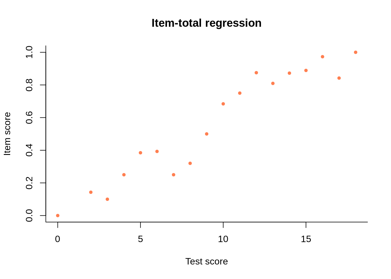
This regression is completely based on observable quantities. On the x-axis we have the possible sum scores from a test of 18 dichotomous items. The expected item score on one of the items (actually, the third), given the sum score, is shown on the y-axis.

It is little to say that item response theory (IRT) is interested in such regressions: in fact, it is made of them – except that it regresses the expected item score on a latent variable rather than the observed sum score. Assuming that each person’s item scores are conditionally independent given the person’s value on the latent variable, and that examinees work independently, we multiply what needs to be multiplied, and we end up with a likelihood function to optimize. Having found estimates for the model parameters, we would like to see whether the model fits the data. In a long tradition going back to Andersen’s test for the fit of the Rasch model, model fit is evaluated by comparing observed and expected item-total regression functions. The item-fit statistics in the OPLM software package (corporate software at Cito developed by Norman Verhelst and Cees Glas), are also of this nature. But the comparison is not necessarily easy – at least, not for every kind of model.

When both variables in a regression are observable, it is equally easy to plot the points that represent the empirical data, or the line that shows what the model predicts for E(Y) given X. Not so when one of the variables is observable but the other one is not. If we keep the latent variable on the x-axis, it is quite easy to plot the model but we don’t know where (at what value of x) to plot the observed data. We can use ability estimates from the model, but there is a touch of circular reasoning in that: we use something that follows from the model to decide whether the model is good. In a regression on observed scores, it is the other way around: there is no problem plotting the observed data (as we did above), but not all models allow us to compute the predicted item score at any given sum score. In fact, among the more popular IRT models, only the Rasch model offers easy computations for this problem. The task is far from trivial with more complicated models. With the 2PL model, we could try a linear interpolation to shrink and stretch axes into an approximate match, but the 3PL model seems logically incompatible with any observable regression.

One of the originalities of dexter is that we have unearthed, in a collected volume on a completely unrelated topic, a model that shares the conditioning property of the Rasch model (RM) while reproducing the empirical data rather faithfully. This is Shelby Haberman’s interaction model (2007), which we have generalized to also handle polytomous items. The briefest way to describe the interaction model (IM) is as a Rasch model with the condition of local independence relaxed. This rich and useful model deserves a separate and more detailed discussion; here, we consider only its most immediate practical utility.

Because of the conditioning property that it shares with the RM, the IM has easy computational rules for the expected score on a given item, given the sum scores on the test. This means that the model predictions can be compared to the empirical data, directly and completely, on a plot or otherwise, without any tricks or approximations. Furthermore, the IM reproduces all features of the data that are psychometrically relevant: the difficulty of the item, its correlation with the test score, and the ability distribution. What is left out is random noise that tends to disappear as the sample size increases. The only snag is that, at the time of writing, we can only fit the IM to complete data, so we cannot use it to calibrate items in a multi-booklet design. Still, the model is invaluable in showing what is in the data, including technical problems otherwise only visible with purely exploratory or non-parametric techniques; and it is a good reference against which to evaluate other models.

Thus, we have two models in dexter. The preferred model for calibrating a test is the extended nominal response model (ENORM), which, as far as the user is concerned, is equivalent to the Rasch model (RM) when all items are dichotomous, and to the partial credit model (PCM), otherwise.¹ To estimate how this model fits the data, we like to compare it with Haberman’s interaction model (IM). In both models, tests are scored with the sum score, based on scoring rules that have been agreed on before we have even seen the data. Both possess the conditioning property, which makes it easy to compare them to each other, and to the empirical data, on a plot file the following one:

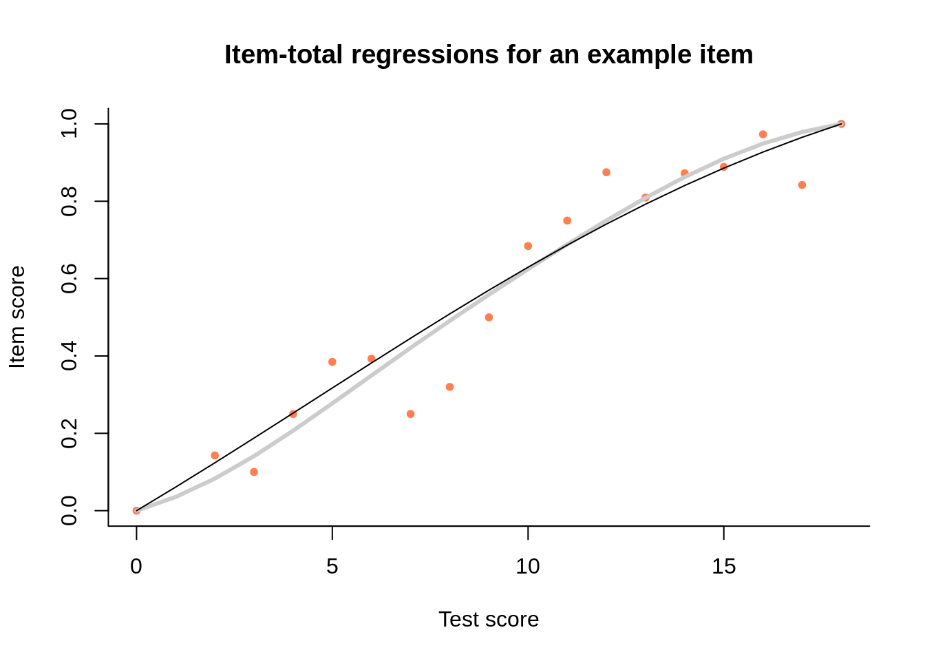
There are three item-test regressions on the plot: the observed one, shown as pink dots; the interaction model, shown with a thick gray line; and the ENORM model, shown with a thin black line. They all share some properties that are worth mentioning:

• All three regressions start at (0,0) because persons with a sum score of 0 must have an item score of 0 for each item; for similar reasons, all regressions end at the point where the maximum item score meets the maximum test score

• The two regression curves cross somewhere in the middle, where most of the data is situated (although the points are plotted in the same size, they represent varying numbers of persons)

• The observed data tends to cluster around the IM regression curve, up to random deviations that diminish with increasing sample size

• Because the IM reproduces faithfully all aspects of the data that are psychometrically relevant, we can actually drop the observed data and assess model fit through the deviation of the RM from the IM. The two regression lines can be compared visually, but we also have a formal Wald test that the interaction parameters in the interaction model are zero. The item-fit statistic, found in the output of function fit_inter, is the estimate of the interaction parameter divided by its standard-error; when the Rasch model holds, it is normally distributed and has the correct type-I error rate.²

Here are some more examples, presented in pairs:

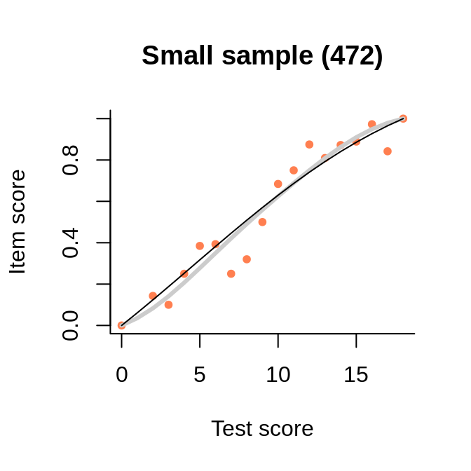
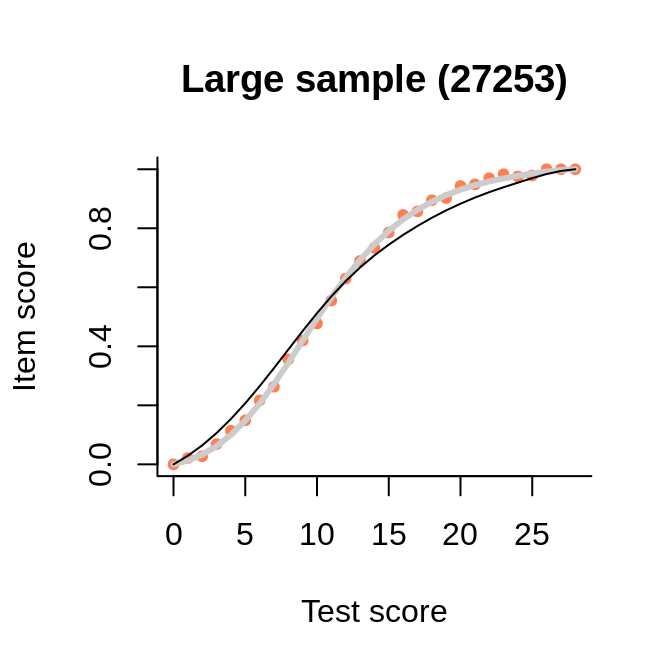
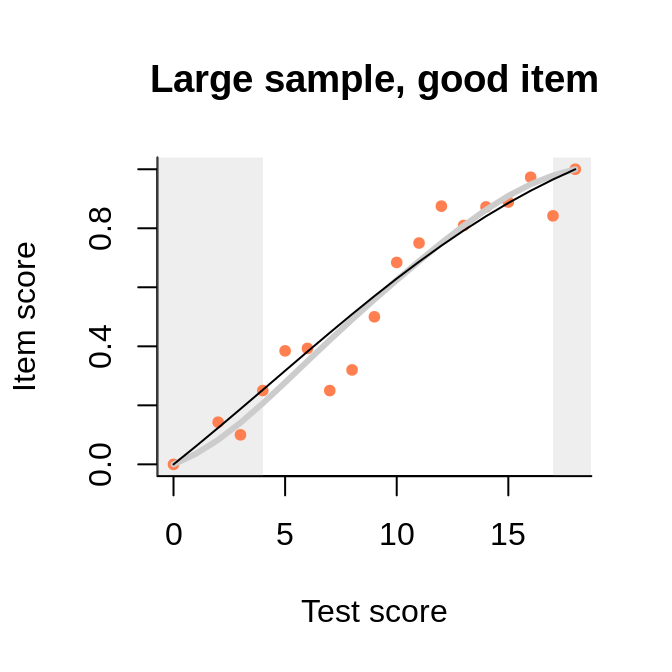
In this example, we see how the points representing the empirical regression cluster more closely around the interaction model (rather than the Rasch model, as long as they differ) when the sample becomes larger.

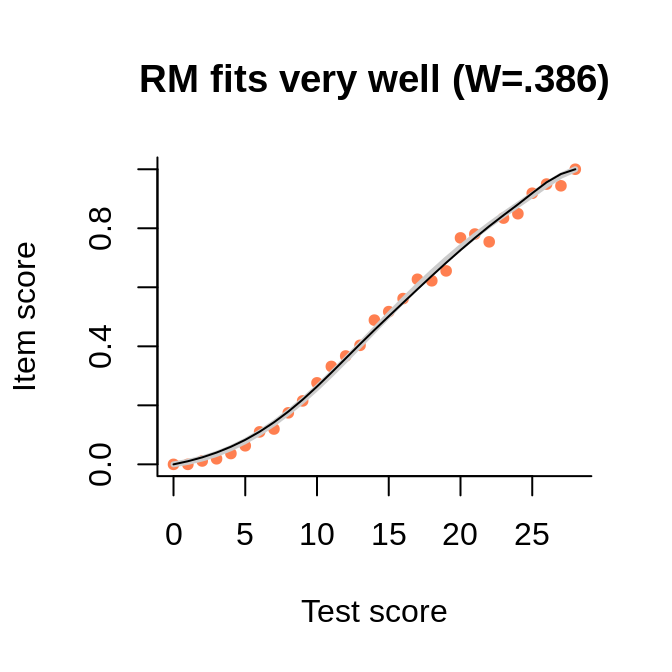
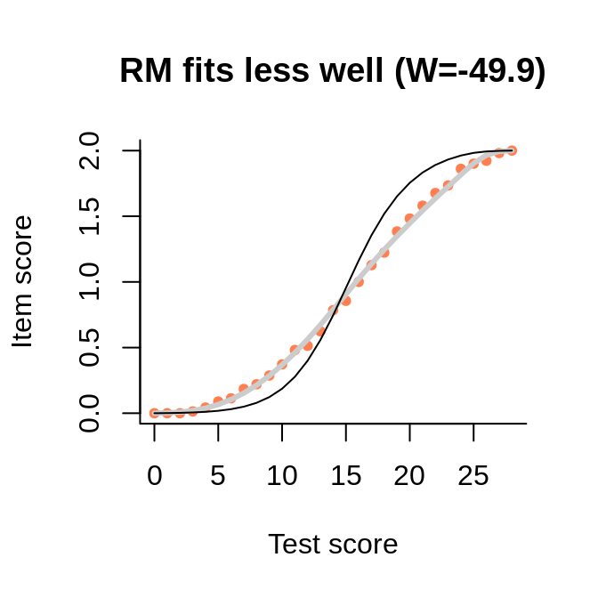
The data comes from the large sample (actually, PISA 2012, one of the mathematics booklets), and the interaction model is very close to the empirical regression. The numbers in the brackets are the Wald tests of fit, to be interpreted as normal deviates.

## 
## rules_changed: 0
## rules_added: 0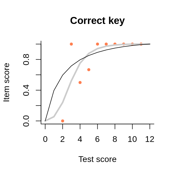

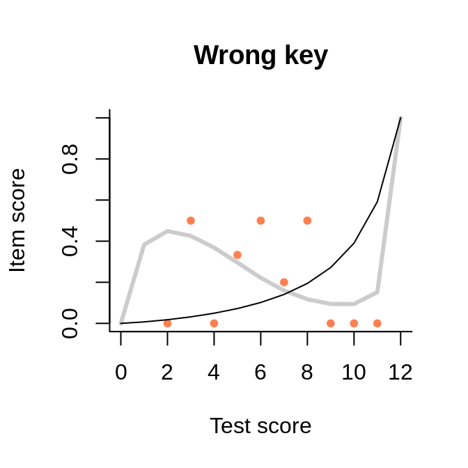
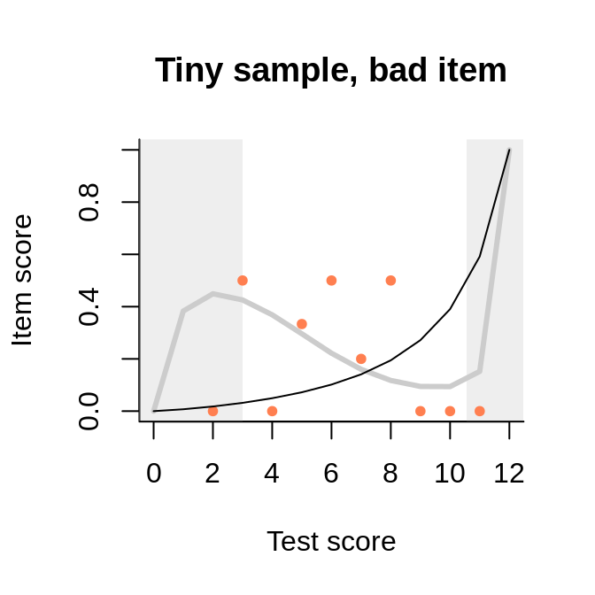
This data set with only 30 persons (probably simulated) has been circulated among publishers of software for test analysis as a test example. The key for one of the items is misspecified, probably on purpose. In spite of the tiny sample and the associated noise in the observed item-total regression, the interaction model represents well the negative slope. Because the regression line is tied at both ends, we see a strange shape akin a cubic polynomial. But the slope is negative where the bulk of the data is situated.

This brings us to one last feature of the plot that we have not explored so far: the curtains. By default, they are drawn at the 5th and the 95th percentile of the observed test scores, highlighting the central 90% of the data:

One purpose of the curtains is to direct our gaze to the part of the plot where the interesting things happen. Another is to give some idea of guessing. We think that this can be approached with the predicted value at an arbitrarily chosen quantile of the raw score distribution – as R. A. Fisher might say, 0.05 seems like a convenient choice. We do have some data there, allowing for a not-too-imprecise estimate, and keeping to the same quantile ensures some statistical comparability across items.

Thus, the left curtain is what we have in lieu of the ‘guessing parameter’. Honestly, we have never particularly liked the 3PL model, which is a curious mixture of two models: one for those who guess and another for those who don’t, so it models the response behavior of no one in particular. The asymptote is notoriously difficult to estimate; if we are not fortunate enough to estimate it without placing a prior, the prior will dominate the estimate entirely as there is practically no data. Finally, the 3PL is incompatible with our regressions. It predicts a positive probability of success at infinitely low ability, but we usually associate minus infinity with a zero score. Zero scores do happen empirically, so at what value of the latent variable do they occur? It cannot be beyond infinity, and if it is nearer than infinity, the regression will not be monotone anymore.

As an example, here is an item with a flat slope and a lot of guessing:

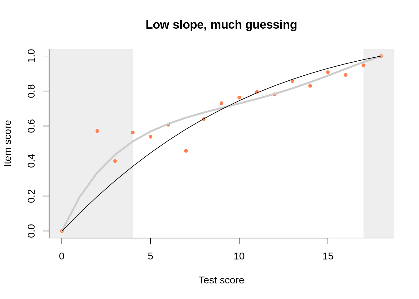
A popular explanation for varying slopes (a.k.a. discriminations) is multidimensionality among the items in the test, but severe deviations tend to be associated primarily with bad item writing. A useful tool in such circumstances is the distractor plot, which is yet another item-total regression: non-parametric and for each possible response to the (closed) item:

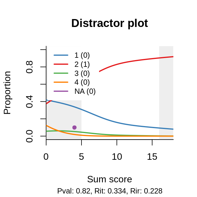
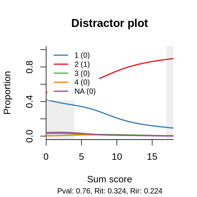
There are two plots because the same item appears in two booklets, but its ‘behavior’ is about the same. Now, of course, if two of our distractors are so weak that even a person of ‘infinitely’ low ability would never pick them, and the only remaining distractor is relatively attractive, we are left with a coin-flipping exercise on the left, and the ‘asymptote’ goes up, predictably, to 0.5. The question is, do we need a special model, with asymptote, as a monument to our bad item writing? To coin yet another paraphrase of Tolstoy’s perennial quote: all good items are similar, all the bad ones are bad in their own way, and the flaws have to be studied and corrected.