Introduction
A critical user of dexter might simulate data and then plot estimates of the item parameters against the true values to check whether dexter works correctly. Her results might look like this:
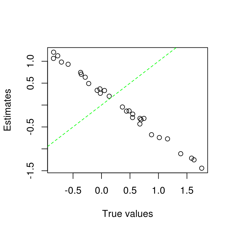
After a moment of thought, the researcher finds that she is looking at item easiness, while dexter reports item difficulties. After the sign has been reversed, the results look better but still not quite as expected:
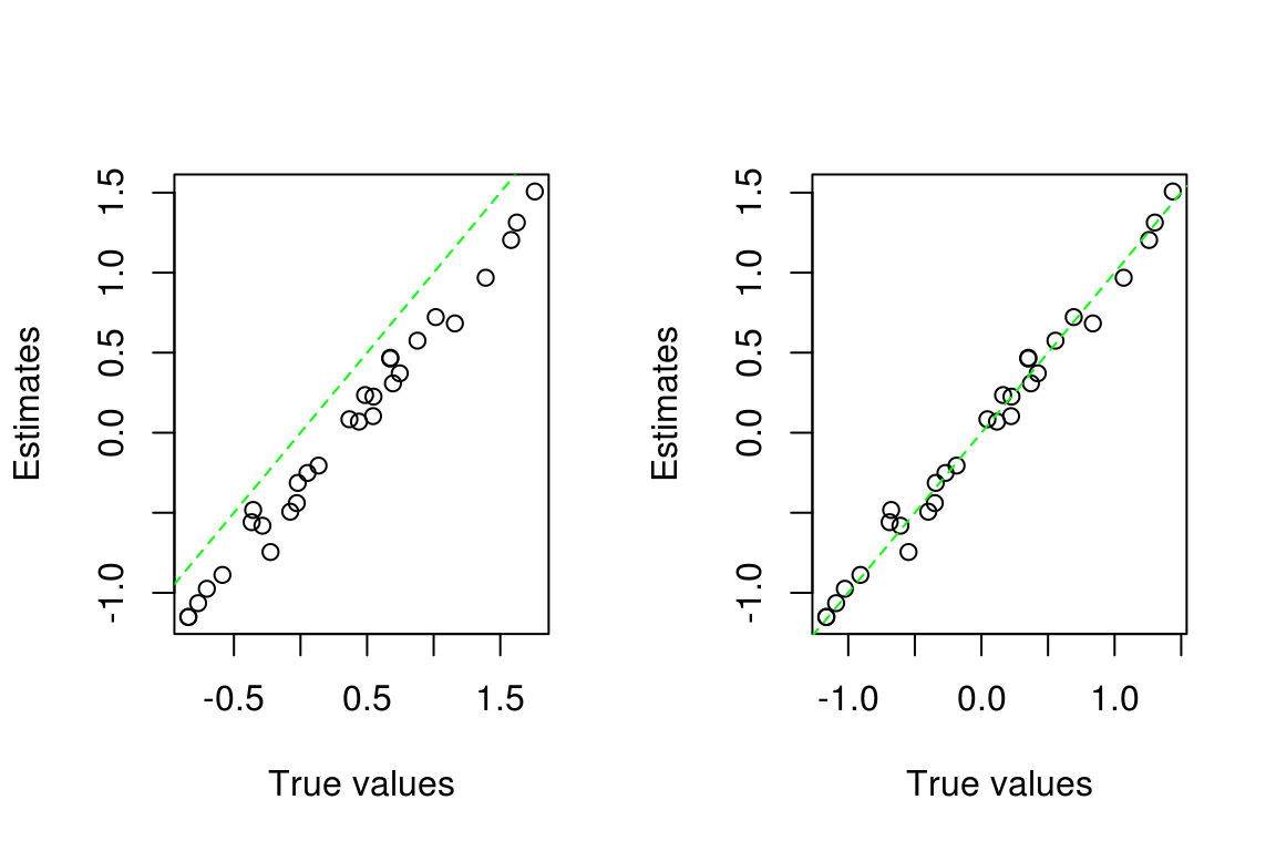
The estimates in the left panel are not clustered around the identity line \(x=y\), and appear to be biased. This time, however, our user notes that dexter reports difficulties relative to the average difficulty, while the true values used to generate the data are relative to the first item. The right panel shows the picture after subtracting the mean from the true estimates. Now things look fine.
This small example illustrates that to interpret parameter estimates a user must know what parameters are reported (that is, one should not compare easiness to difficulty), and on which scale. The first issue is that of parameterization, while the second refers to what is usually called normalization i.e., what restrictions are imposed to identify the model.
Parameterization
For simplicity, consider the Rasch model. dexter uses the following parameterization to communicate to users:
\[ P(X_i = 1 |\theta, \beta_i) = \frac{\exp(\theta-\beta_i)}{1+\exp(\theta-\beta_i)}, \] where \(\theta\) represents person ability and \(\beta_i\) the difficulty of item \(i\); both parameters are real-valued. This parameterization is used for communication because it prevails in the literature. Besides, \(\beta_i\) has an appealing interpretation as the value of ability where an incorrect and a correct answer are equally likely; that is, \(P(X_i = 0 | \beta_i, \beta_i) = P(X_i = 1 | \beta_i, \beta_i) = 1/2\).
Internally, Dexter uses a different parameterization: \[ P(X_i=1|t,b_i) = \frac{tb_i}{1+tb_i} \]
where \(t = \exp(\theta)\) and \(b_i = \exp(-\beta_i)\) and both positive real numbers. This parameterization is more convenient for estimation.
The two expressions for the Rasch model look quite different but they describe the same model: for any \((\theta, \beta_i)\), there exist unique values \(t\) and \(b_i\) that give the same likelihood. We can use either one as we see fit. In any event, our user will have to make sure that she compares \(\beta\) to \(\beta\), and not apples to … kiwis?
Normalization
In the Rasch model, abilities and item difficulties are on the same scale but the origin of the scale is arbitrary. This is because \(\theta^* = \theta - c\) and \(\beta^*_i = \beta_i - c\), for any constant \(c\), give the same probabilities and thus the same likelihood such that, empirically, all values of c are (equally) good. More technically, the origin is said to be not identifiable from the observations. No amount of data will tell us what the origin should be.
Differences between items and/or persons are identified because they are independent of the origin, \(c\). It follows that the common scale can be depicted as a line with estimated item difficulties and abilities as locations. As this image, sometimes called an item map, easily becomes cluttered, we show an example with only a few arbitrarily chosen items and persons:
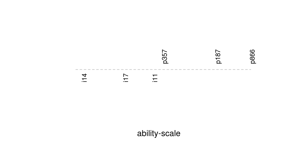
We have been careful to not put any numbers on the item map. This is because the origin is arbitrary, and so would be the numbers.
To assign values to the parameters, we choose an arbitrary origin by imposing a restriction called a normalization. dexter uses two normalizations, both on the item parameters. During estimation, the first item parameter is set to zero, i.e., \(\delta_1 =0\), or \(b_1 = 1\). For reporting, the package follows the OPLM tradition and sets the mean item difficulty to zero, i.e., \(\sum_i \delta_i = 0\). The latter implies that estimates (i.e., abilities and difficulties) must be interpreted as relative to average difficulty.
Comparing ability distributions
That the latent scale has an arbitrary origin is well-known but, at the same time, easily overlooked. Consider an investigator who wishes to compare 15-year olds in two subsequent years; each group is given a test containing a set of common items called the anchor.
The researcher analyses the data from both years separately and looks at the ability distributions.
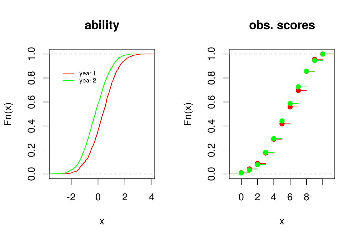
The ability distributions differ and it seems that pupils have changed. If, however, we look at the observed scores on the anchor, we see no difference in their distribution. How, then, can pupils change in ability yet score equally? Have the items become easier? Again, we simulated the data such that we know the answer: the change in ability is actually a change in scale and should not to be taken to mean that the groups differ. More precisely, in each analysis the origin is the average difficulty. The origins differ because the items differ. In practice, one may not be aware of this.
To avoid the problem, we have two options. The first is to analyse data from the second year fixing the parameters of the anchor items at the values found in the previous year. The second is to analyze the data simultaneously. The results are as follows:
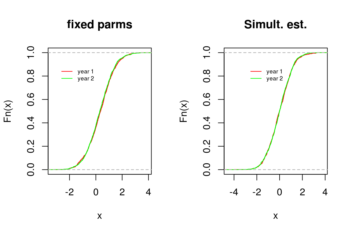
In both cases, the pictures now show that the distributions are indeed equal. Note that we can test whether the distributions are equal using a Kolmogorov-Smirnov test but this will be left for some other occasion.
If we must choose, we would much prefer to estimate the parameters using all available data. If we fix the parameters of the anchor items at the values found in the first year, we do not make use of the responses on these items collected in the second year. This means that we willingly ignore information. Furthermore, we allow idiosyncrasies of the first sample to bias the results of future years. In general, the more data, the better the estimates.
The idea to fix the parameters of the anchor items may have come up because it is convenient to have estimates of abilities and item parameters on the same scale, even when the item set changes over years. But, if the purpose is to fix the scale, there is no need to fix the difficulties of the anchor items. We can achieve the same if we fix, for example, the origin at the average ability in the first year.
Conclusion
Using a simplified context for illustration, we have tried to explain what it means that the ability scale in IRT does not have a definite origin. In closing, we advise researchers to avoid looking at things that are not identified by the observations. These include differences between items and persons and functions of these such as the item-total regressions or, indeed, the difference between ability distributions of different groups of respondents. Even than one should not forget that we are doing statistics and there is uncertainty in the estimates.