We could have issued a WARNING: This bag package is not a toy! But we can do better. In a series of posts, we will discuss how to use dexter to analyze data from large scale educational assessments, such as PISA. The task is a rather imposing one, not only in the amount of data to be crunched, but mostly in the number of issues to discuss.
In this first part, we will analyze the mathematics domain in PISA 2012 (OECD 2014). With 65 participating countries, 21 booklets and over half a million of students, this is anything but a toy example. We will focus on the basics: how to obtain the data, get it into dexter, estimate the parameters of the IRT model, compute plausible values, and apply survey weights and variance estimation. With these technical aspect under the belt, we can concentrate on more conceptual issues in further blogs.
Obtain and parse PISA data and get it into dexter
As of the time of writing, the following works. We believe that the OECD will keep the data available forever; however, minute changes in the exact location cannot be excluded, and that would necessitate changes in the code.
We need two files: the scored cognitive item response data file, and the student questionnaire data file. We will first focus on the responses to the cognitive items. The student questionnaire file will be needed later for the survey weights and plausible values it contains.
The first step is to download the scored cognitive item response data file from the PISA website. This is a compressed text file; to unzip it, we follow the steps suggested by Koohafkan (2014).
library(dexter)
library(tidyverse)
library(SAScii)
url1 = "http://www.oecd.org/pisa/pisaproducts/INT_COG12_S_DEC03.zip"
url2 = "http://www.oecd.org/pisa/pisaproducts/PISA2012_SAS_scored_cognitive_item.sas"

zipfile = 'cogn.zip'
download.file(url1, zipfile)
fname = unzip(zipfile, list=TRUE)$Name[1]
unzip(zipfile, files = fname, overwrite=TRUE)
Next, parse the data into a data frame (a tibble, to be more precise) by using the SAS control file and the parse.SAScii() function from the SAScii package. For the sake of simplicity, we recode both codes for missing values (i.e., 7 for N/A, and 8 for ‘not reached’) to NA, although we admit that it could be worth to pay more attention to the structure of the missing values. This is, however, beyond the scope of this paper.
dict_scored <- parse.SAScii(sas_ri = url2)
unlink(zipfile)

data_scored <- read_fwf(
  file = fname,
  col_positions = fwf_widths(dict_scored$width, col_names = dict_scored$varname)) %>%
  select(CNT, SCHOOLID, STIDSTD, BOOKID, starts_with('PM'))

unlink(fname)

data_scored$BOOKID = sprintf('B%02d', data_scored$BOOKID)
data_scored[data_scored==7] = NA
data_scored[data_scored==8] = NA
Note that we selected a subset of the data (all math items have variable names starting with PM). Now, start a new dexter project and add the data. First we need to declare all items and their admissible scores in a rules object. We pass that to the start_new_project function.
rules = gather(data_scored, key='item_id', value='response', starts_with('PM')) %>%
  distinct(item_id, response) %>%
  mutate(item_score = ifelse(is.na(response), 0, response))

head(rules)
## # A tibble: 6 x 3
## item_id response item_score
## <chr> <int> <dbl>
## 1 PM00FQ01 NA 0
## 2 PM00FQ01 0 0
## 3 PM00FQ01 1 1
## 4 PM00GQ01 NA 0
## 5 PM00GQ01 0 0
## 6 PM00GQ01 1 1db = start_new_project(rules, "pisa2012.db", covariates=list(
cnt = '<unknown country>',
schoolid = '<unknown country>',
stidstd = '<unknown student>'
)
)Now we can add the data, booklet by booklet:
data_scored %>%
  group_by(BOOKID) %>%
  do({
    rsp = select_if(., function(x) !all(is.na(x)))
    booklet_id = .$BOOKID[1]
    add_booklet(db, rsp, booklet_id)
    data.frame()
  })
## # A tibble: 0 x 1
## # Groups: BOOKID [0]
## # ... with 1 variable: BOOKID <chr>rm(data_scored)At some later stage, we will discuss a market basket approach to the definition and estimation of competence (Mislevy 1998; Zwitser, Glaser, and Maris 2017). For our purposes, the market basket is the subset of items that is administered in every country (though not to every student, as we have a multi-booklet design within each country). We are not dealing with the market basket approach now, but we will compute an item property, ‘item belongs / does not belong to the basket’, and we will add it to the data base for later use:
item_by_cnt = get_responses(db, columns=c('person_id', 'item_id', 'item_score', 'cnt')) %>%
  group_by(cnt,item_id) %>%
  summarise()

market_basket = Reduce(intersect, split(item_by_cnt$item_id, item_by_cnt$cnt))

item_properties = dbGetQuery(db, "SELECT item_id FROM dxItems") %>%
  mutate(in_basket = item_id %in% market_basket)

add_item_properties(db, item_properties)
## 1 item properties for 109 items added or updatedOur data base is complete now (took only a couple of minutes), and we can, and should, do some exploratory analysis to assess the quality of the items and identify possible problems. In a PISA study, this step is usually done at national level, and involves the computation of various statistics derived from classical test theory (CTT). dexter has excellent facilities for this kind of analysis, but they are best employed in interactive mode. The two interactive functions, iTIA and iModels, are set up such that all vital computations are performed at the beginning. This means that, with a survey of this size, one must wait for about a minute for a CTT analysis of all booklets, including test and item level statistics and distractor plots; after that, results can be browsed without noticeable delay. The waiting time for a deeper analysis of a separate booklet, including the three item-total regressions, is about a couple of seconds.
Unfortunately, interactive analysis is difficult to demonstrate in a static paper. The interested readers can try them out by themselves. Alternatively, they could use the new package, dextergui, which makes interactive analysis even easier.
Fit the IRT model
The IRT model in dexter is not exactly the same as the one used in the original PISA study of 2012. PISA used the Mixed Coefficients Multinomial Logit Model (Adams, Wilson, and Wang (1997)), which is a multidimensional model fit by marginal maximum likelihood (MML). The extended nominal response model (ENORM) in dexter is a unidimensional model fit by conditional maximum likelihood (CML). Still, there is an essential structural similarity: both models default to the Rasch model for the dichotomous items, and to the partial credit model (PCM) items for the polytomous items.
CML estimation tends to be fast:
system.time({item_parms = fit_enorm(db)})## ==## user system elapsed
## 69.082 1.276 70.704Compute plausible values
Plausible values (PV) are random draws from the posterior distribution of a person’s ability, given the item parameters and the person’s responses (Maarten Marsman (2014)). Nowadays, they are the standard method of ability estimation when studying populations (when testing individuals in a high stakes exam, we typically use the expectation of the posterior rather than a random draw).
The plausible values in the original PISA study are drawn with a prior distribution that reflects a large number of background variables measured on the person. We don’t do this. A wonderful property of PV values is that they eventually reproduce the true ability distribution, even when the prior is misspecified (M. Marsman et al. (2016)). Using the wrong prior comes with a penalty: one must pay with more data, meaning more items. When the functional form of the posterior resembles the functional form of the prior, this is a sign that convergence is near.
The algorithm used in dexter is based on composition (sample a proposal value, simulate data from it, accept if the simulated sum score matches the observed one), and uses recycling for higher speed (rejected values are saved for some other persons). See Maarten Marsman (2014) for details.
system.time({pv = plausible_values(db, parms=item_parms, nPV=5)})## user system elapsed
## 80.297 1.090 81.615head(pv)## booklet_id person_id sumScore PV1 PV2 PV3
## 1 B01 dxP1 7 -0.42229867 -0.6786812 -1.450302899
## 2 B01 dxP10 2 -2.31743257 -2.2179755 -2.980653556
## 3 B01 dxP100 7 -1.41020927 -0.9710605 0.001638266
## 4 B01 dxP1000 12 -0.02766521 -0.1706592 0.064511598
## 5 B01 dxP10000 8 -0.89955379 -0.5194595 -0.555766694
## 6 B01 dxP10001 9 -0.71979277 -0.5272382 -1.531430362
## PV4 PV5
## 1 -1.2091211 -1.4695097
## 2 -2.9724133 -2.5534355
## 3 -1.0925180 -0.9166020
## 4 -0.8380541 -0.4751191
## 5 -0.4204032 -0.8081987
## 6 -0.3742272 -0.4861613Note that we could have omitted the parms argument, in which case the IRT model will be estimated automatically. Once we have set up the dexter data base, PISA’s original approach, or a good approximation, takes one line of code!
Survey weights and variance estimation
Large-scale studies like PISA make every effort to represent faithfully particular populations. They use scientific sampling, which, for efficiency reasons, does not necessarily give every student in the population the same probability to be selected. As long the sampling probabilities are known, the potential bias can be neutralized by weighting the individuals’ data with (essentially) the inverse of these probabilities. The weights are also adjusted to reduce the biasing effect of nonresponse.
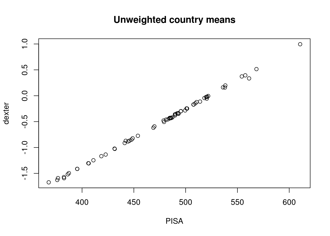
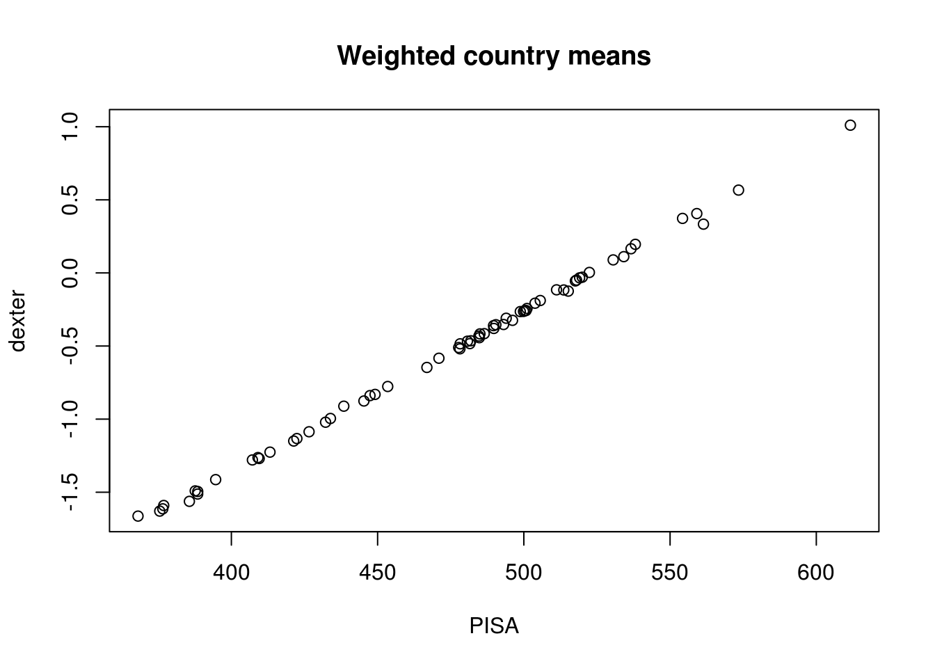
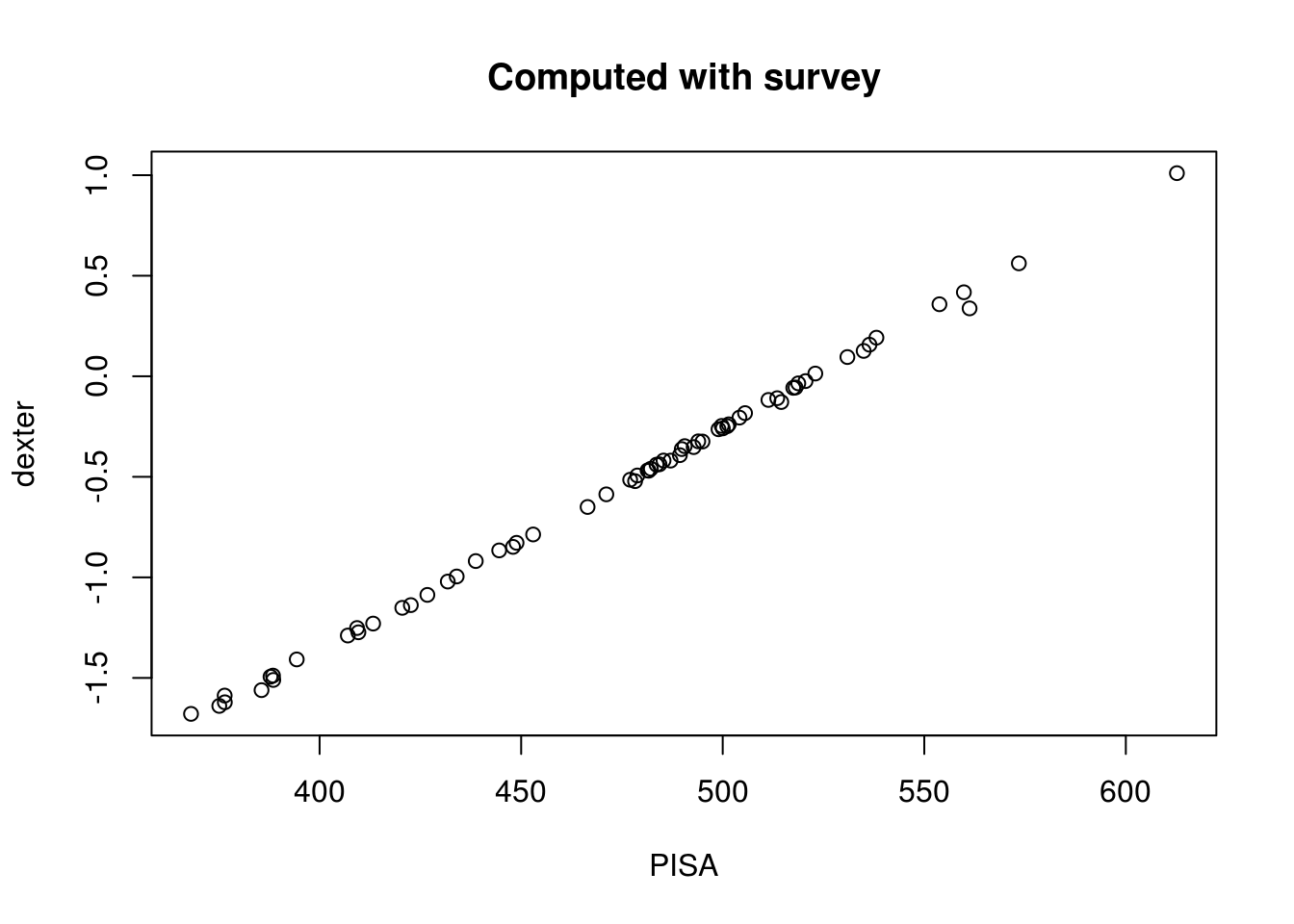
Actually, we don’t need the weights to compare our PV to PISA’s original ones. But, for didactic purposes, and to get done with all technicalities before proceeding to more conceptual issues, we will do three comparisons: unweighted, weighted, and exactly as in PISA.
First, download the student questionnaire file, which contains, along with a huge amount of background data, PISA’s plausible values, and the sampling and replicate weights necessary to compute the estimates and their standard errors. The operations are similar to those we used to get the cognitive response data:
url3 = 'http://www.oecd.org/pisa/pisaproducts/INT_STU12_DEC03.zip'
url4 = 'http://www.oecd.org/pisa/pisaproducts/PISA2012_SAS_student.sas'

zipfile = 'quest.zip'
download.file(url3, zipfile)
fname = unzip(zipfile, list=TRUE)$Name[1]
unzip(zipfile, files = fname, overwrite=TRUE)

dict_quest = parse.SAScii(sas_ri = url4)

dict_quest = parse.SAScii(sas_ri = url4) %>%
   mutate(end = cumsum(width),
          beg = end - width + 1) %>%
   filter(grepl('CNT|SCHOOLID|STIDSTD|PV.MATH|^W_FST', varname))

data_quest = read_fwf(file = fname, fwf_positions(dict_quest$beg, dict_quest$end, dict_quest$varname))

unlink(zipfile)
unlink(fname)
We have selected the variables containing the country (CNT), the school and the student IDs, the five plausible values, and a large number of variables whose name starts in W_FST; the latter contain sampling and replicate weights.
From the dexter data base, extract student identification variables and add them to our freshly generated PV, so we can match these with PISA’s PV:
ids = get_persons(db)
scores = ids %>%
  left_join(pv, by='person_id') %>%
  setNames(toupper(names(.))) %>%
  inner_join(data_quest)
Using just the first PV out of five, compare unweighted and weighted country means:
means = scores %>%
  group_by(CNT) %>%
  summarise(
    uD = mean(PV1),
    uP = mean(PV1MATH),
    wD = weighted.mean(PV1, w=W_FSTUWT),
    wP = weighted.mean(PV1MATH, w=W_FSTUWT)
  )
plot(means$uP, means$uD, main='Unweighted country means', xlab='PISA', ylab='dexter')
plot(means$wP, means$wD, main='Weighted country means', xlab='PISA', ylab='dexter')
To estimate country means and their standard estimates as in PISA, we use package survey (Lumley (2004)). First, we make a replication design with W_FSTUWT as sampling weights, and the many variables whose names start in W_FSTR as replicate weights:
library(survey)
ds =  svrepdesign(repweights = '^W_FSTR',
      weights = ~W_FSTUWT,
      combined.weights = TRUE,
      data = scores)
rm(scores,ps1,ps2,pv,ids,data_quest)
The following function will do all computations explained in the PISA Technical Manual. Essentially, we compute, for each country and for each of the five PV, a large number of differently weighted means. The replicate weights are chosen such that, in each replication, the data for half of the schools is ignored while the data for the other half is doubled; the replications differ in which schools fall into the two halves. The uncertainty due to having a sample of schools and students rather than the whole population is reflected in the differences between replications, while the uncertainty due to psychometric measurement is reflected in differences between the five PV. The two kinds of error, sampling variance and imputation variance, are then combined with a simple formula (see the arrow in the code):
pvby = function(formula, by, design, FUN, ...) {
   npv = length(attr(terms(formula),"term.labels"))
   m   = 1 + 1 / npv
   est = svyby(formula, by, design, FUN, ...)
   nv = attr(est,"svyby")$nstats
   e  = coef(est)
   ne = length(e)
   d  = c(ne %/% nv, nv %/% npv, npv)
   e = array(e, dim = d)
   v = array(SE(est)^2, dim = d)
   estimate = apply(e, 1:2, mean)
   sampvar  = apply(v, 1:2, mean)
   impuvar  = apply(e, 1:2, var)
   stderr   = sqrt(sampvar + m * impuvar) # <======
   rownames(estimate) = rownames(stderr) = rownames(SE(est))
   colnames(estimate) = paste("stat", 1:ncol(estimate), sep = "")
   colnames(stderr) = paste("SE", 1:ncol(stderr), sep = "")
   res = cbind(estimate, stderr)
   res
}
We use this function twice to get estimates and standard errors for the plausible values computes with dexter and for PISA’s original estimates:
res_pv   = pvby(~PV1+PV2+PV3+PV4+PV5,~CNT,ds,svymean)
res_pisa = pvby(~PV1MATH+PV2MATH+PV3MATH+PV4MATH+PV5MATH,~CNT,ds,svymean)
plot(res_pisa[,1], res_pv[,1], main='Computed with survey', xlab='PISA', ylab='dexter')
Obviously, and in spite of some minor technical differences, the plausible values estimated with dexter produce almost the same results as the original PISA survey of 2012. This is nice, but it is neither surprising nor sensational. Having explained, step by step, how to compute with a large data set we are now ready to discuss what to compute, and why: a more entertaining discussion that will be taken up in the next posts.
References
Adams, R.J., M. Wilson, and W. Wang. 1997. “The Multidimensional Random Coefficients Multinomial Logit Model.” Applied Psychological Measurement 21 (1): 1–23.
Koohafkan, Michael. 2014. “Downloading, Extracting and Reading Files in R.” February. https://hydroecology.net/downloading-extracting-and-reading-files-in-r/.
Lumley, Thomas. 2004. “Analysis of Complex Survey Samples.” Journal of Statistical Software 9 (1): 1–19.
Marsman, M., G. Maris, T. M. Bechger, and C. A. W. Glas. 2016. “What can we learn from plausible values?” Psychometrika, 1–16.
Marsman, Maarten. 2014. “Plausible Values in Statistical Inference.” PhD thesis, Enschede, the Netherlands: University of Twente.
Mislevy, R. J. 1998. “Implications of Market-Basket Reporting for Achievement-Level Setting.” Applied Psychological Measurement 11 (1): 49–63.
OECD. 2014. “PISA 2012: Technical Report.” http://www.oecd.org/pisa/pisaproducts/pisa2012technicalreport.htm.
Zwitser, Robert J., S. Sjoerd F. Glaser, and Gunter Maris. 2017. “Monitoring Countries in a Changing World: A New Look at Dif in International Surveys.” Psychometrika 82 (1): 210–32. doi:10.1007/s11336-016-9543-8.