In an enormously influential short paper, Embretson (1996) sums up five most important differences between classical test theory (CTT) and item response theory (IRT). The first among them is that, in CTT, the standard error of measurement applies to all scores in a particular population, while in IRT the standard error of measurement differs across scores, but generalizes across populations.

To see how this works, we first take a leisurely, informal look at some simple examples with the Rasch model; we then examine the information functions more formally, and we explain how they are implemented in dexter.

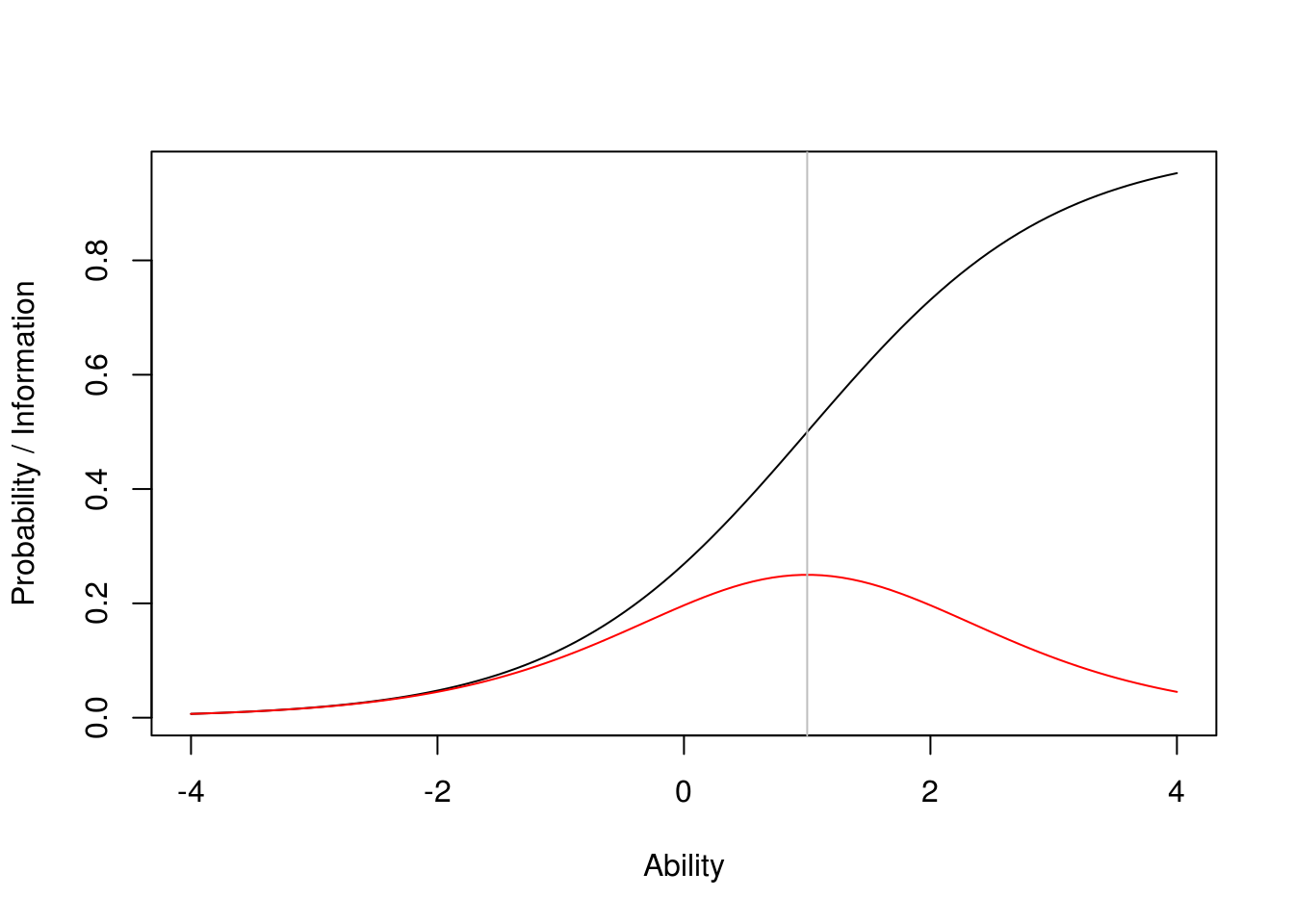
The Rasch model predicts that, given an item and its difficulty parameter, \(\beta\), the probability of a correct response is a logistic function of ability, \(\theta\), namely, \[P(\theta;\beta)=\frac{\exp(\theta-\beta)}{1+\exp(\theta-\beta)}.\] The information function for the same item happens to be \(P(\theta;\beta)[1-P(\theta;\beta)]\), so it is, again, a function of \(\theta\). Below we show the item response curve (IRF) for the item, i.e., the function \(P(\theta;\beta)\) along with the corresponding item information function (IIF), shown in red. When \(\theta=\beta\), \(P(\theta;\beta)=0.5\); this is also the point where the IIF peaks, and the maximum is of course equal to 0.25.

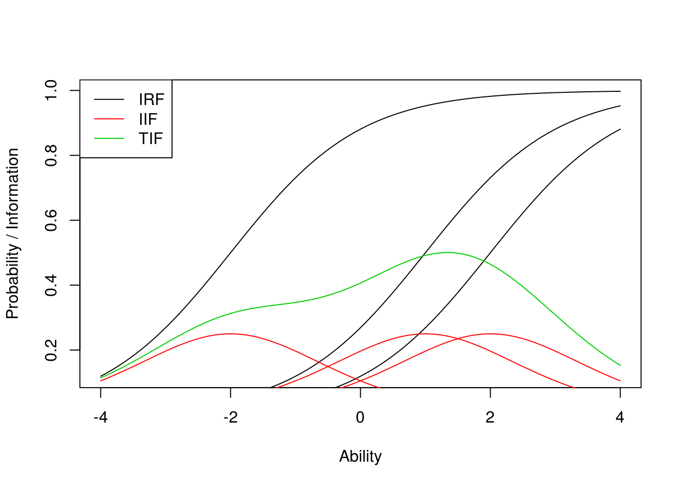
Now, the test information function (TIF) is, simply, the sum of the IIF over all items in the test. Under the Rasch model, this is a function of \(\theta\) bounded between 0 and \(1/4\) the number of items in the test. Now, the standard error of measurement (SEM) is inversely related to the TIF. More precisely, \(\text{SEM}=\sqrt{1/\text{TIF}}\), so it is again a function of \(\theta\), and it appears that it cannot go lower than \(2/\sqrt{k}\) with \(k\) the number of items in the test.

This is all illustrated with three items on the plot below. In IRT, we have a clearer idea of planning our test and its precision. To get the error of measurement more even over the ability range, we should have items of various difficulties included. If, on the contrary, we are interested in maximizing measurement precision near some important threshold where decisions are made, it would make sense to include more items with difficulties in that particular range. And, the idea of adaptive testing is just around the corner.

That was the easy introduction, now follows the more interesting part. Let us stage the actors:

First, there is the IRT model. Let \(X_i\) denote the response to item \(i\) with \(X_i=j\) the event that the \(j\)th response was chosen corresponding to a score \(a_{ij}\). In dexter, the basic IRT model is the NRM, which is a divide-by-total model and can be written as: \[ P(X_{i} = j |\theta) = P_{ij}(\theta) = \frac{ F_{ij}(\theta)}{\sum_h F_{ih}(\theta)} \] where \(F_{ij}(\theta) = b_{ij} e^{a_{ij}\theta}\) is a positive increasing functions of student ability \(\theta\) with derivatives: \[ \frac{d F_{ij}(\theta)}{d \theta} = a_{ij} F_{ij}(\theta), \text{and} \\ \frac{d}{d\theta} \ln P_{ij}(\theta) = a_{ij} - \sum_h a_{ih}P_{ih}(\theta) \]

The second actor is the log-likelihood function. It is useful to define \(x_{ij}\) as a dummy-coded response with \(x_{ij} = 1\) if \(X_i=j\) and zero otherwise. This allows us to write the log-likelihood with respect to ability as: \[ \ln L(X_i|\theta) = \sum_j x_{ij} \ln P_{ij}(\theta) \] with derivatives \[ \frac{d}{d\theta} \ln L(X_i|\theta) = \sum_j x_{ij}\left(a_{ij} - \sum_h a_{ih}P_{ih}(\theta)\right) \]

The item information function is what statisticians call the (observed) Fisher information of an item response variable \(X_i\) about \(\theta\) (see Ly et al. (2017)). It can be defined as: \[\begin{align*} I_{i}(\theta) &= - \frac{d^2}{d\theta^2} \ln L(x_i|\theta) \\ &= \sum_j a_{ij} P_{ij}(\theta)\left[\frac{d}{d\theta} \ln P_{ij}(\theta) \right] \\ &= \sum_j a_{ij} P_{ij}(\theta)\left(a_{ij} - \sum_h a_{ih} P_{ih}(\theta) \right) \end{align*}\]

Finally, the test information function is simply the sum of the item information functions; i.e., \[ I(\theta) = \sum_i I_{i}(\theta). \] Since item information is just test information when the test consists of one item, we need only consider how to calculate test information. To do the calculations efficiently we write \[ I_i(\theta) = \sum_j a_{ij} P_{ij}(\theta) a_{ij} - \left(\sum_j a_{ij} P_{ij}(\theta)\right)^2 \] This inspires the following implementation, where first and last are vector of indices. That is, the parameters of each item are ordered with first indicating where (in vectors \(\mathbf{b}\) and \(\mathbf{a}\)) they start and last where they end.

myIJ = function(b, a, first, last, theta)
{
  nI=length(first)
  I = matrix(0,nI, length(theta))
  for (i in 1:nI)
  {
    Fij = b[first[i]:last[i]]*exp(outer(a[first[i]:last[i]],theta))
    Pi = apply(Fij,2,function(x)x/sum(x))
    M1 = Pi*a[first[i]:last[i]]
    M2 = M1*a[first[i]:last[i]]
    I[i,] =  colSums(M2) - colSums(M1)^2
  }
  colSums(I)
}

To use myIJ, we run fit_enorm and take out the item parameters, \(\mathbf{b}\), the item scores, \(\mathbf{a}\), and the vectors first and last from the output. We will from now on use the user-level function which does this for us.

As an example, let us calculate the information function using a real-data example. We first get the data from a test (no, we are not telling you which), and we estimate the item parameters using female respondents who took booklet 1652 (geslacht means gender in Dutch):

db = open_project("670.db")
prms = fit_enorm(db, booklet_id=="1652" & geslacht=="f")

## =

The next step is to calculate the information function and plot it.

Inf_1652 = information(prms, booklet = "1652")
plot(Inf_1652, from=-4,to=4, main = "booklet 1652", 
                             ylab = "test information",
                             xlab = "Ability")

## plot in standard-error of max. likelihood estimator of ability
abls=ability_tables(prms)
points(abls$theta,1/abls$se^2,pch=16, cex=0.5, col="blue")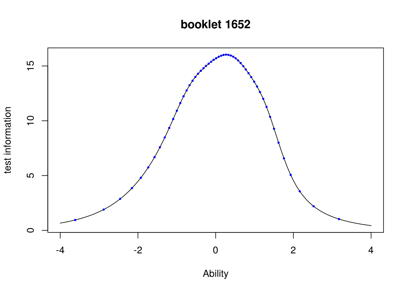

The points on the curve correspond to \(1/se(\theta)^2\), where \(se\) is the standard-error of the maximum-likelihood estimate (MLE) of ability. This illustrates the relationship \(1/\sqrt{I(\theta)} = se(\theta)\) between the standard error of the MLE and test information given ability \(\theta.\) The plot shows that the test is most suited for respondents whose true abilities lie around \(0.3\).

It is worth noting that information returns a function. Thus, to get the test information at \(\theta=0\), one would simply type Inf_1652(0). The ability corresponding to maximum information can be found using optimize(Inf_1652,c(-4,4), maximum = TRUE); in this case 0.2750423.

In practice, item parameters are not known. Let us repeat the exercise but this time taking the uncertainty about the item parameters into account. To this effect, we first estimate the item parameters using a Bayesian method.

prms = fit_enorm(db, booklet_id=="1652" & geslacht=="f", 
                 method = "Bayes", nIterations = 515)

## ===========================================================================

The number of iterations, 515, is the number we need to produce a posterior sample of size 100 if we use a burn-in of 20 and thereafter choose every fifth-th sample to get rid of auto-correlations.

plot(Inf_1652, from=-4,to=4, main = "booklet 1652", 
                             ylab = "test information",
                             xlab = "Ability")
for (i in seq(from=20,to=15+5*100,by=5))
{
  Inf_ = information(prms, booklet = "1652", which.draw = i)
  plot(Inf_, from=-4,to=4, add=TRUE, col="grey")
}
plot(Inf_1652, from=-4, to=4, add=TRUE)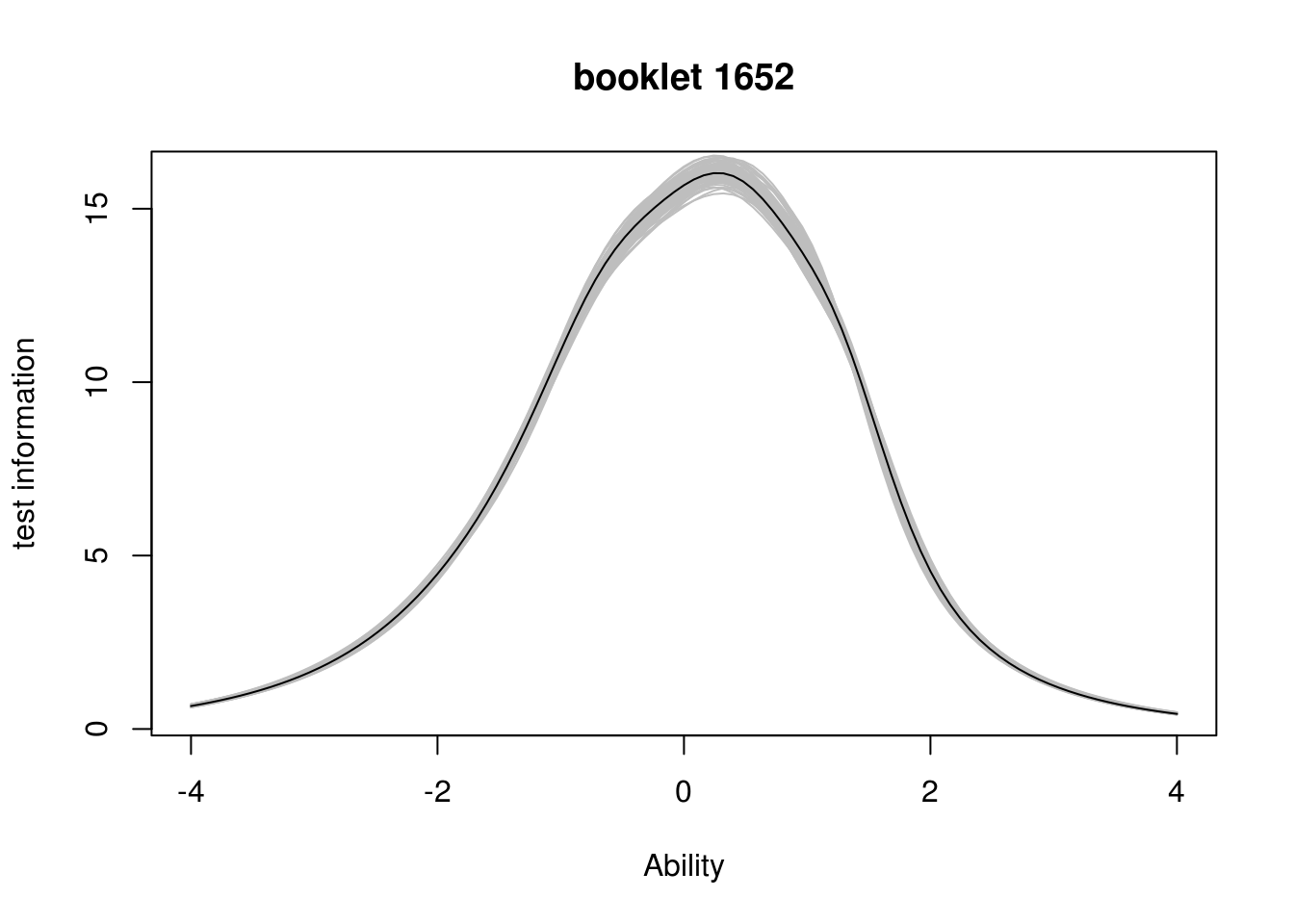

The shape of the curve is well-preserved but note that, even with as many as 5753 respondents, the information function is clearly affected by uncertainty in the item parameters.

References

Embretson, Susan. 1996. “New Rules for Measurement.” Psychological Assessment 8 (4): 341–49.
Ly, Alexander, Maarten Marsman, Josine Verhagen, Raoul PPP Grasman, and Eric-Jan Wagenmakers. 2017. “A Tutorial on Fisher Information.” Journal of Mathematical Psychology 80. Elsevier: 40–55.