In my post on DIPF from yesterday, I had plots with an arbitrary aspect ratio chosen automatically by R. Rather than change them behind the scenes, I revisit them because I feel the issue deserves attention.
To start with the MDS plot: it is supposed to reconstruct a map from a distance matrix, so there is no discussion that the aspect ratio should be set to 1 by adding asp=1 to the arguments of the plot function. Like this:
plot(mmds$points, type='n', xlab='Dimension 1', ylab='Dimension 2', asp=1)
text(mmds$points, rownames(mmds$points), cex=.6)
abline(h=0, col='gray')
abline(v=0, col='gray')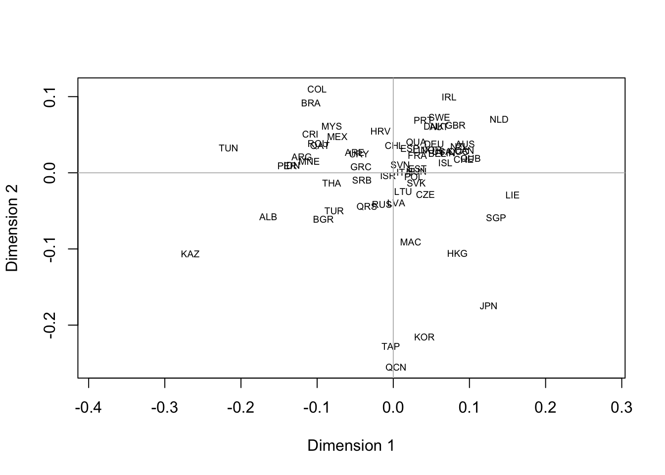
What about the PCA? There is not much sense in dividing the eigenvectors by the square root of the eigenvalues if R is going to rescale them again, using some arbitrary value. So, the plot of the first and second components should really look like this:
plot(spl[,1], spl[,2], ty="n",
     xlab="First PC", ylab="Second PC", asp=1)
text(spl[,1], spl[,2], names(dimat), cex=.6)
segments(0, 0, spl[,1], spl[,2], col='gray')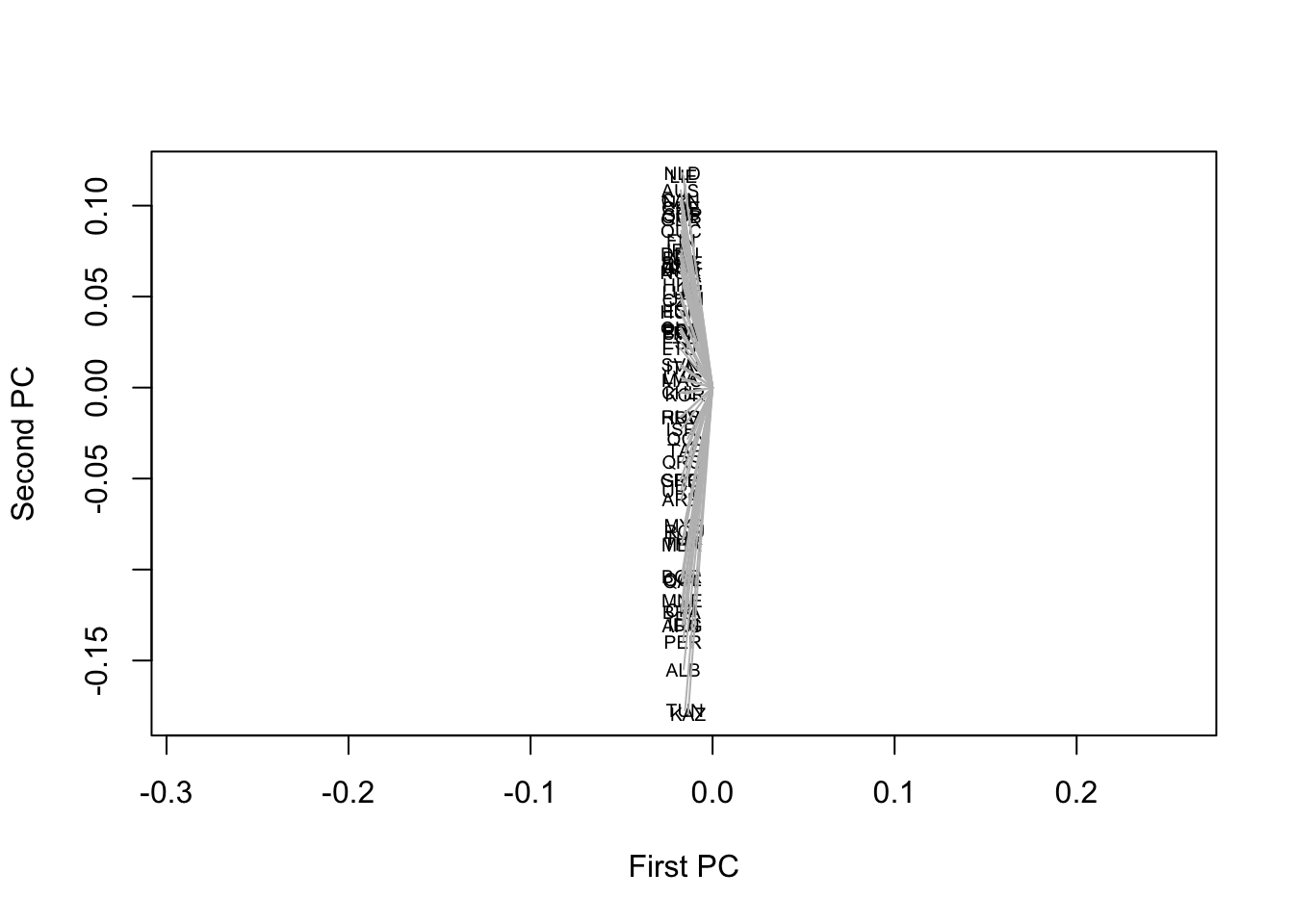
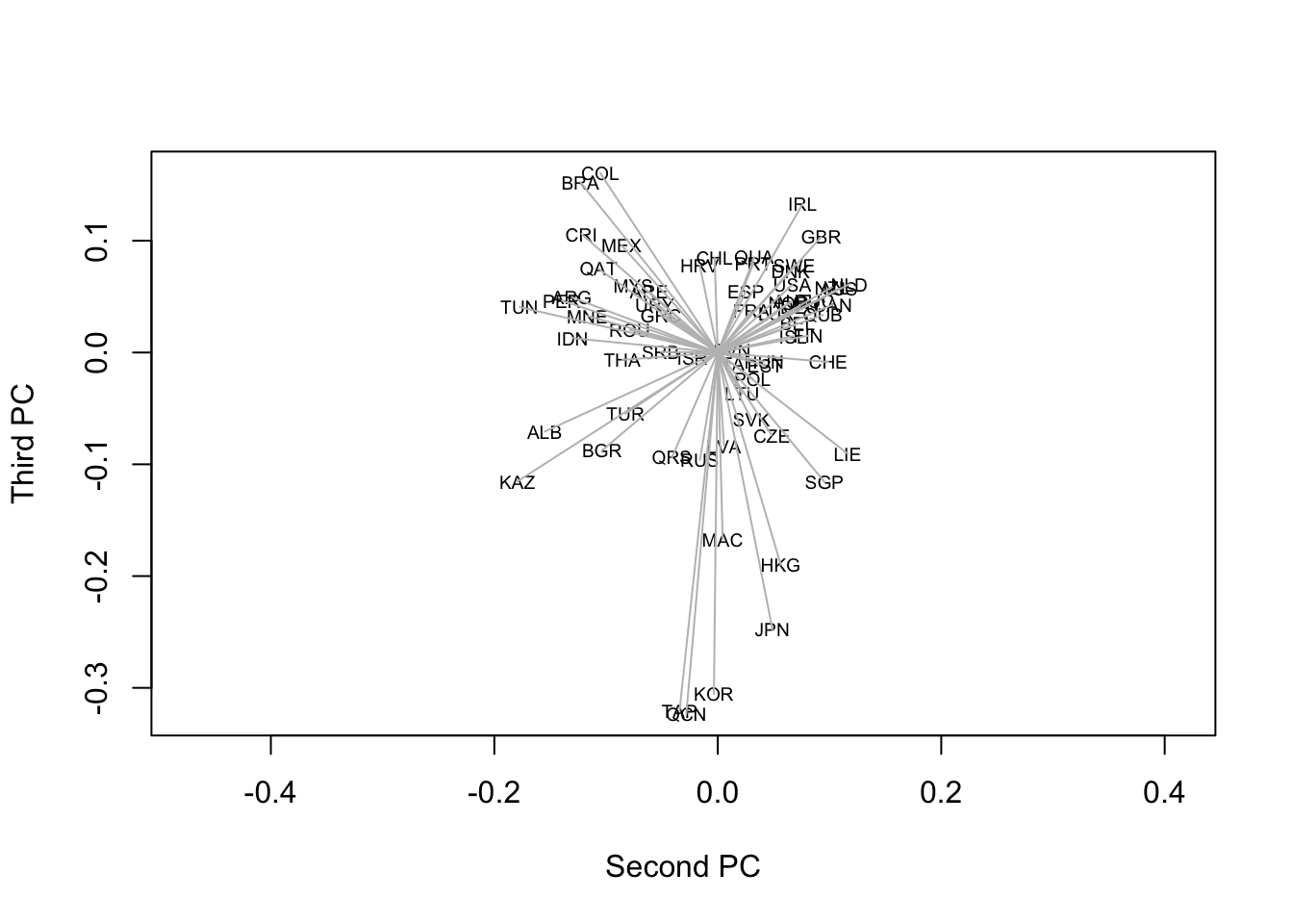
Not very helpful perhaps – the slight misfit of some Asian countries on the first axis is more difficult to detect – but there is an objective truth in it about the strength of the first principal component (which vanished as we transformed the similarities into dissimilarities). For the second and third components:
plot(spl[,2], spl[,3], ty="n",
     xlab="Second PC", ylab="Third PC", asp=1)
text(spl[,2], spl[,3], names(dimat), cex=.6)
segments(0, 0, spl[,2], spl[,3], col='gray')