Local (in)dependence and polytomization

dexter has a function, fit_domains, that deals with subtests. Domains are subsets of the items in the test defined as a nominal variable: an item property. The items in each subset are transformed into a large partial credit item whose item score is the subtest score; the two models, ENORM and the interaction models, are then fit on the new items.

To illustrate, let us go back to our standard example, the verbal aggression data. Each of the 24 items pertains to one of four frustrating situations. Treating the four situations as subtests or domains, we obtain for one of them:

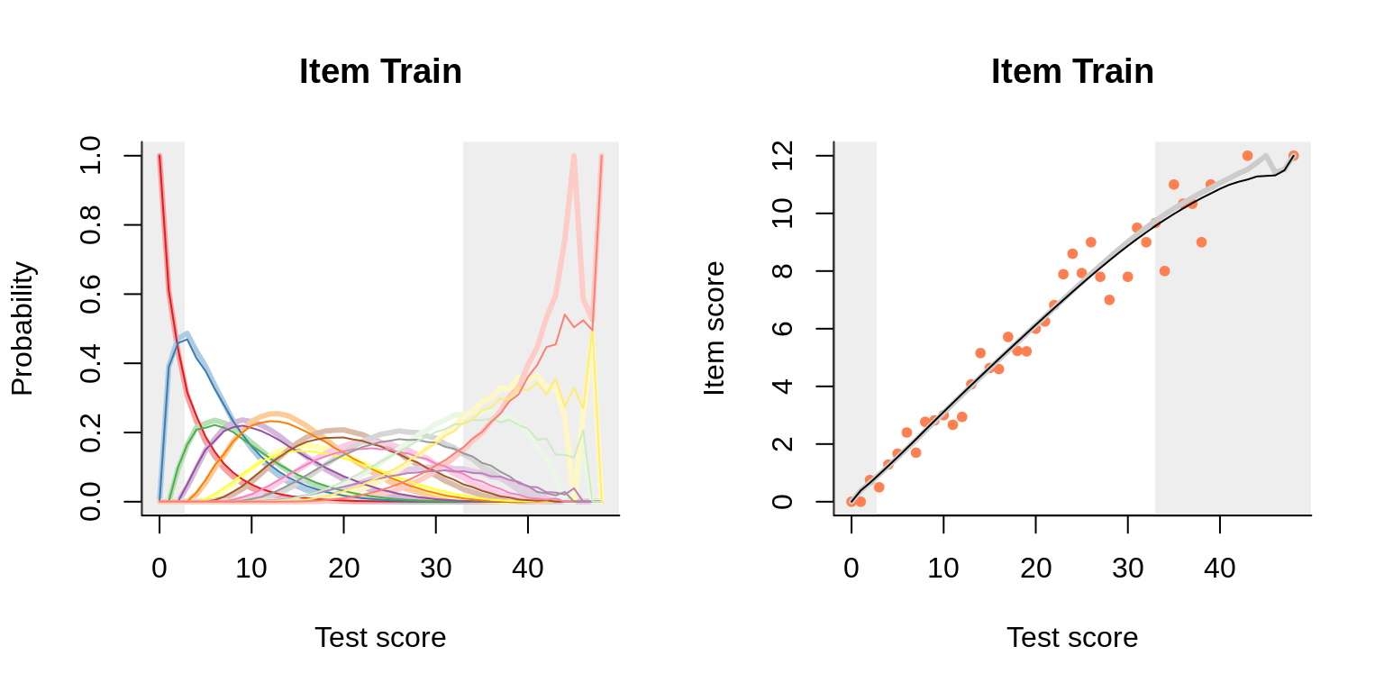
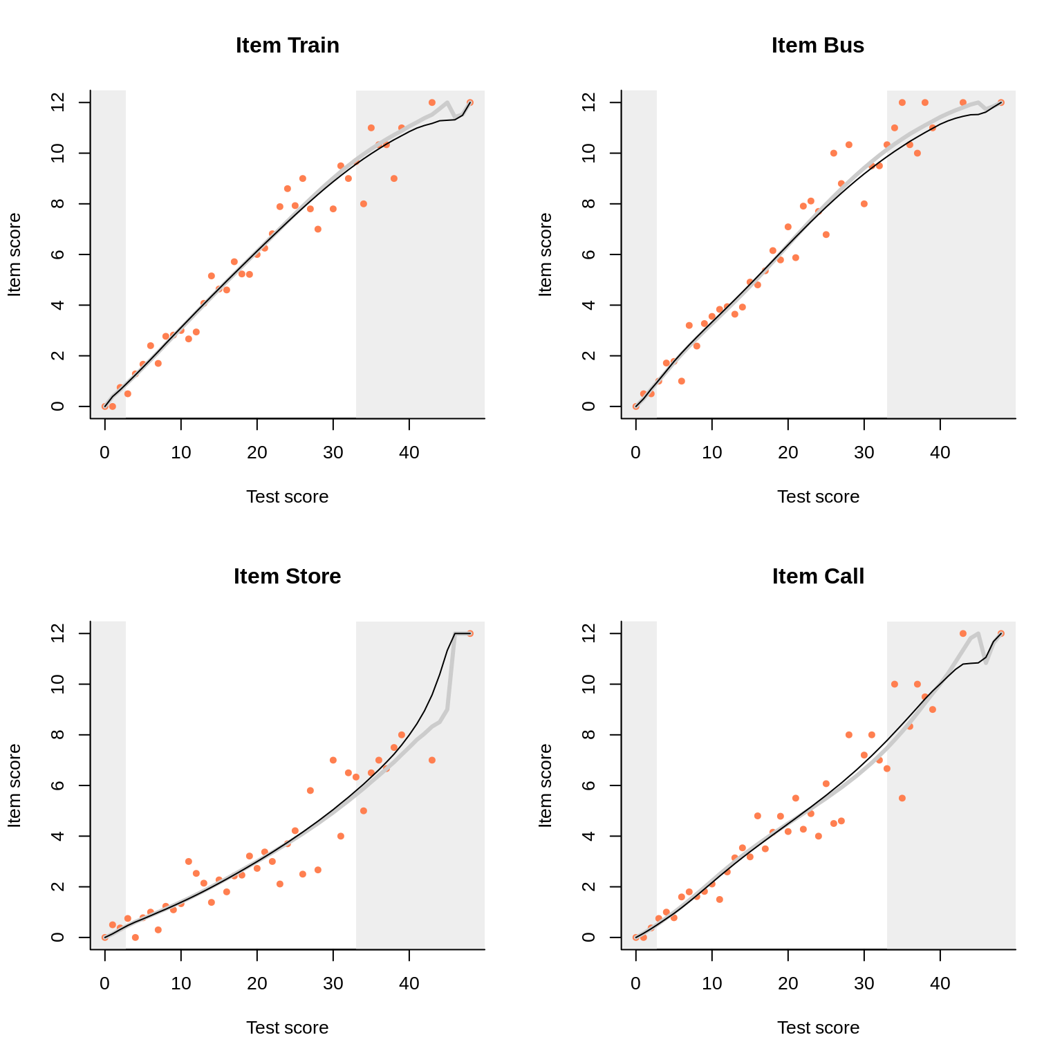
To the left we see how the two models compare in predicting the category probabilities; to the right are the item-total regressions for the item (i.e. domain) score. Everything looks nice for this high-quality data set, but note in particular how closely the two models agree for the domain score. For all four situations:

Observations like these are ubiquitous. After all, the (polytomous) interaction model differs from ENORM in allowing for local dependence, and there is a certain tradition in dealing with local dependence through polytomization. We will review this tradition here, bearing in mind that its potential is probably far from exhausted. To spice things up even more, we will consider rated data.

The assumption of local stochastic independence (LSI) can be violated for many reasons. One example is when raters grade various aspects of the examinee’s work. The rubric may have the grading on one aspect depend on the grading on other aspects. Or there may be a halo effect: raters assign lower grades to an aspect if they have assigned higher grades to other aspects. To make matters concrete, suppose that an examinee has written an essay that is rated by rater \(g\) on three aspects using rubric \(s\). We assume a one-point rubric: each aspect is graded \(0\) if insufficient and \(1\) if sufficient. Consider a model where the probability of the three grades, \(\mathbf{x}_{g}=(x_{g1},x_{g2},x_{g3})^{t}\), given \(\theta\) can be expressed as \[ \Pr(\mathbf{x}|\theta,\beta_{1},\beta_{2},\beta_{3},\beta_{sg})\propto \exp(r\theta - \sum_{a=1}^{3}x_{a}\beta_{a}-x_{1}x_{3}\beta_{sg}) \] In this equation \(r\) denotes the number of aspects that were judged sufficient. It is seen that the probability depends on \(x_1,x_2,x_3\), and on the combination of \(x_1\) and \(x_3\). This is a special case of a model described by Kelderman (1984).

Now consider the grades assigned to different aspects as independent items such that \[ \Pr(X_{a}=x_{a}|\theta,\beta_{a})\propto\exp(x_{a}(\theta-\beta_{a})),\quad x_{a}=0,1. \] Given LSI, the probability of a response pattern \(\mathbf{x}_{g}\) is given by \[ \prod_{a=1}^{3}\Pr(X_{a}=x_{a}|\theta,\beta_{a}) \propto \exp(r\theta-\sum_{a=1}^{3}x_{a}\beta_{a}) \] which is equal to our model for rated data if \(\beta_{sg}=0\). Thus, the parameter \(\beta_{sg}\) models the violation of LSI due to the rater (subscript \(g\)) or the scoring rubric (subscript \(s\)). In this example, it is assumed that grades given to the first aspect and the third aspect are related given \(\theta\), but more complex dependencies can be modeled by a straightforward extension of the model.

Under the Kelderman model, the probability of a score \(r\) is modeled as \[\begin{align*} \Pr(R=r|\theta,\beta_{1},\beta_{2},\beta_{3},\beta_{sg}) &=\sum_{\mathbf{y}:\sum_{i}y_{i}=r}\Pr(\mathbf{x}|\theta,\beta_{1},\beta_{2},\beta_{3},\beta_{sg})\\ & \propto\sum_{\mathbf{y}:\sum_{i}y_{i}=r}\exp(r\theta-\sum_{a=1}^{3}y_{i}\beta_{a}-y_{1}y_{3}\beta_{sg})\\ & \propto\exp(r\theta)\sum_{\mathbf{y}:\sum_{i}y_{i}=r}\exp(-\sum_{a=1}^{3}y_{a}\beta_{a}-y_{1}y_{3}\beta_{sg}) \end{align*}\] The second term is positive and, given the beta parameters, it depends only on \(r\), the rubric \(s\), and the rater \(g\). Hence, we can write this factor as \(\zeta_{rsg}\). If we define \(\eta_{rsg}\equiv-\ln(\zeta_{rsg})\) we can write \[ \Pr(R=r|\theta,\beta_{1},\beta_{2},\beta_{3},\beta_{sg})\propto \exp(r\theta)\exp(-\eta_{rsg})=\exp(r\theta-\eta_{rsg}) \] This model is formally equivalent to a PCM with \(\eta_{0sg}=\ln(1)\) \(=0\) for all raters \(g\) and all \(s\). Thus, polytomizing releases us of the need to model local dependencies. Hence, this is one reason why model fit improves when we polytomize. It will be clear that the same argument would hold if the original items follow an interaction model.

The argument has been worked out in greater generality by Verhelst and Verstralen (2008) who note that local dependencies can still be seen if we look at the item-category parameters of the polytomized items. Suppose that LSI holds and \(\beta_{sg}=0\). In that case we find that \(\eta_{rsg}=\eta_{r}\) for all raters \(g\). In addition, it can be shown that certain order relations must hold among the category parameters. To see this, we stay in the context of the example and define \(b_{i}\equiv \exp(-\beta_{i})\). We may then write \[\begin{align*} \eta_{r} &=-\ln\left[ \sum_{\mathbf{y}:\sum_{i}y_{i}=r}\exp(-\sum_{i=1}^{3} y_{i}\beta_{i})\right] \\ & =-\ln\left[ \sum_{\mathbf{y}:\sum_{i}y_{i}=r}\prod_{i=1}^{3}\exp(-\beta_{i})^{y_{i} }\right] \\ & =-\ln\left[ \sum_{\mathbf{y}:\sum_{i}y_{i}=r}\prod_{i=1}^{3}b_{i}^{y_{i} }\right]\\ & =-\ln\gamma_{r}(b_{1},b_{2},b_{3}) \end{align*}\] where \(\gamma_{r}(b_{1},b_{2},b_{3})\) is the usual way to denotes the elementary symmetric function of order \(r\) with argument \((b_{1},b_{2},b_{3})^{t}\). Thus, under LSI the same relationships that hold between elementary symmetric functions of different orders hold between the PCM parameters; e.g., the classical Newton inequalities. Verhelst and Verstralen (2008) propose to test whether these relations hold.

References

Kelderman, Hendrikus. 1984. “Loglinear Rasch Model Tests.” Psychometrika 49 (2). Springer: 223–45.
Verhelst, Norman D, and HHFM Verstralen. 2008. “Some Considerations on the Partial Credit Model.” Psicologica: International Journal of Methodology and Experimental Psychology 29 (2). ERIC: 229–54.