When we apply IRT to score tests, we most often use a model to map patterns of TRUE/FALSE responses onto a real-valued latent variable, the great advantage being that responses to different test forms can be represented on the same latent variable relatively easy. When all observed responses are continuous, most psychometricians will probably think first of factor analysis, structural equations and friends. Yet the world of IRT is more densely populated with continuous responses than anticipated.
To start with, computer-administered testing systems such as MathGarden readily supply us with pairs of responses and response times. It is a bit awkward to model them simultaneously, since responses are usually discrete (with few categories) and response times continuous – yet there exist a myriad of models, as the overview in Boeck and Jeon (2019) shows. To apply the same type of model to both responses and response times, Partchev and De Boeck (2012) have chosen to split the latter at the median, either person- or item-wise.
Second, item responses increasingly get scored by machine learning algorithms (e.g. Settles, T. LaFlair, and Hagiwara (2020)), whose output is typically a class membership probability. If classification is to be into two classes, the boundary is usually drawn at 0.5. One of the questions we ask ourselves in this blog is whether there can be a better way.
Within more traditional testing, there have been attempts to avoid modeling guessing behavior with ad hoc models by asking test takers about their perceived certainty that the chosen response is correct (Finetti (1965), Dirkzwager (2003)). These approaches also lead to responses that can be considered as continuous.
The Rasch model for continuous responses must have been proposed many times in more or less obvious forms. As represented, for example, in Verhelst (2019):
\[ f(x_i|\theta) =\frac{\exp(x_i[\theta-\delta_i])}{\int^1_0 \exp(s(\theta-\delta_i)) ds} \]
where \(x_i\) is the (continuous) response to item \(i\), \(\theta\) is the latent ability, and \(\delta_i\) is an item difficulty parameter. The similarity with the conventional Rasch model is obvious, except that we are now predicting a density rather than a probability. The assumption of local independence plays just as important a role, i.e., we can multiply over items to get at the likelihood for the entire response pattern. The integral in the denominator has a closed form:
\[\begin{equation*} \int^1_0 \exp(s(\theta-\delta_i)) ds = \begin{cases} \frac{\exp(\theta-\delta_i)-1}{\theta-\delta_i} & \text{if $\theta \neq \delta_i$} \\ 1 & \text{if $\theta = \delta_i$} \end{cases} \end{equation*}\]
The model – we shall call it henceforth the continuous Rasch model, or CRM – is an exponential family model; like the Rasch model, it has the property that the person and item sum scores are sufficient statistics for the model parameters: the student ability, \(\theta\), and the item difficulty, \(\delta_i\). Models discussed in Maris and Maas (2012) and Deonovic et al. (2020) can be shown to have the same structure.
In this blog, we capitalize on new insights in Deonovic et al. (2020) and Maris (2020) to demonstrate how the CRM can be used for any type of continuous responses. We show how to plot the density, the probability function, and the expectation under the CRM, how to simulate data from it, and we explore the limits to which dexter can be used to analyze continuous responses (hint: we plan to push these limits with a new package in the near future).
Density, probability function, and expectation of the CRM
These can be calculated easily in R with the following functions:
# probability density function
dCR = function(x, eta=2)
{
  if (eta==0) 1
  if (eta!=0) eta*exp(x*eta)/(exp(eta)-1)
}

# cumulative distribution function
pCR = function(x,eta)
{
  (exp(x*eta)-1)/(exp(eta)-1)
}

# Expectation
ECR = function(eta)
{
  dm = exp(eta)
  dm = dm/(dm-1) - 1/eta
  dm[is.na(dm)] = 0.5
  dm
}
The following graph shows them for various choices of \(\eta_i=\theta-\delta_i\):

Note that the expected score is monotone increasing in student ability, as it should be.
Simulating data from the CRM
Simulated data conforming to the CRM can be generated by inversion sampling. Specifically,
\[ P(x_i \leq x) = \begin{cases} \frac{e^{x\eta_i}-1}{e^{\eta_i}-1} & \text{if $\eta_i \neq 0$}\\ x & \text{if $\eta_i \neq 0$} \end{cases} \] where \(x \in [0,1]\). This means that if we sample \(u\) from a uniform distribution, \[ u^* = \begin{cases} \frac{1}{\eta} \log\left(u(e^\eta - 1) + 1\right) & \text{if $\eta \neq 0$}\\ u & \text{if $\eta \neq 0$} \end{cases} \] is an item response sampled from the CRM.
Sampling from the CRM can be thus done with a single line of code:
rCR = function(theta, delta)
{
  eta = theta - delta
  ifelse(eta!=0, (1/eta)*log(runif(nrow(X))*(exp(eta)-1)+1), runif(nrow(X)))
}
The following code produces a data set in long format with 5000 persons answering to 100 items.
n <- 100 #number of items
N <- 5000 #number of persons
delta <- runif(n, -1, 1) #difficulty
theta <- rnorm(N, 0, 1) #ability

X <- data.frame(person_id = rep(1:N, each=n),
                 item_id = rep(1:n, N))

X$response = rCR(theta[X$person_id], delta[X$item_id])
Analyzing a binary response derived from the continuous one
At the time of writing, dexter has no provision to deal with continuous responses. Instead, we use the suggestion by Deonovic et al. (2020) to analyze binary responses derived from the continuous ones. How does this work?
With \(x_i\) an observed continuous response, define two new variables:
\[ \begin{align} y_{i1}&=(x_i>0.5) \\ x_{i1}&= \begin{cases} x_i-0.5 & \text{ if } y_{i1}=1 \\ x_i & \text{ if } y_{i1}=0 \end{cases} \end{align} \]
These are conditionally independent sources of information on ability from which the original observations can be reconstructed; that is, given \(\theta\), \(Y_{i1}\) is independent of \(X_{i1}\). Moreover, it is easy to show that the implied measurement model for \(Y_{i1}\) is the Rasch model:
\[ p(Y_{i1}=1|\theta)=p(X_i>0.5|\theta) = \frac{\exp(0.5(\theta-\delta_i))} {1+\exp(0.5(\theta-\delta_i))} \]
where the discrimination is equal to 0.5. The other variable, \(X_{i1}\), is continuous and has the following distribution over the interval 0 to \(1/2\):
\[\begin{equation} f(x_{i1}|\theta) = \frac{(\theta-\delta_i)\exp(x_{i1}(\theta-\delta_i))}{\exp(0.5(\theta-\delta_i))-1} \end{equation}\]
Thus, both \(X_{i1}\) and \(X_i\) follow a CRM but the former has a different range for the values of the continuous response.
The proposal is to analyze the constructed dichotomous responses instead of the original continuous responses. The following code makes these responses and fits the Rasch model to them:
library(dexter)
Z = X
Z$item_score = 1*(Z$response > 0.5)
f = fit_enorm(Z)
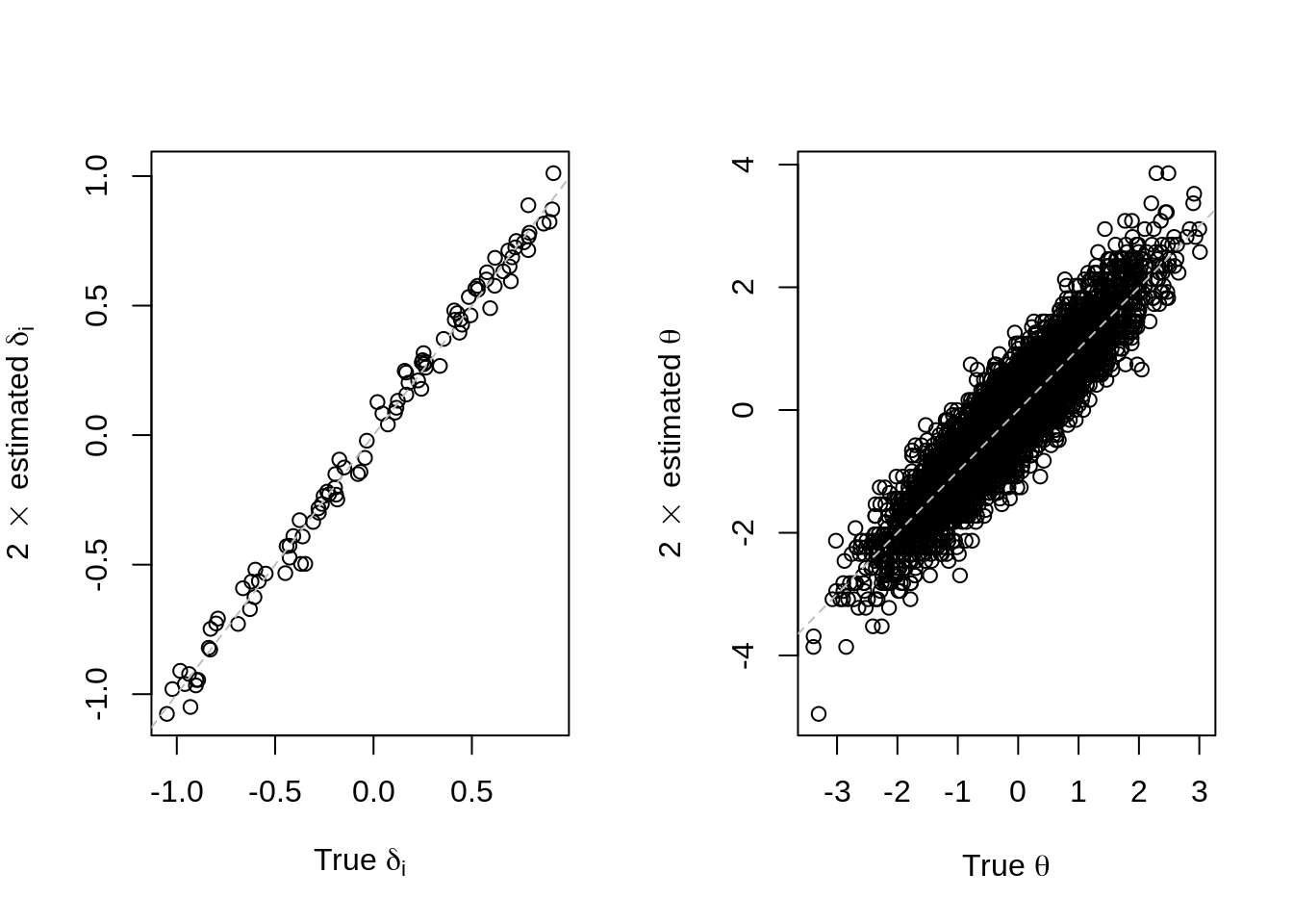
Let us see whether we recover the parameters:

Obviously, parameter recovery was quite good. Note that the discrimination was specified as 1, as a half is not allowed in dexter – thus, we estimate twice the abilities and difficulties that have been used to generate the data.
Dyadic expansion
We can continue the process and split up \(x_{i1}\) into two new variables, \(y_{i2}\) and \(x_{i2}\), then split up \(x_{i2}\), and so on. In this way, we recursively transform the continuous response intto a set of conditionally independent Rasch response variables, \(y_{i1}, y_{i2}, \dots\). Deonovic et al. (2020) note that this corresponds to the dyadic expansion of \(x_i\); that is,
\[ x_i = \frac{y_{i1}}{2^1} + \frac{y_{i2}}{2^2} + \frac{y_{i3}}{2^3} + .. \]
The discrimination will halve in every step of the recursion, which means that each new item provides (four times) less information about ability than its predecessor. More specifically, the information function of the dyadic expansion of order \(d\) can be defined as:
\[ I^{(d)}_i(\theta) = \sum^d_{j=1} I_{ij}(\theta) \] where \[ I_{ij}(\theta) = \frac{1}{2^{2j}} \pi_{ij}(\theta)(1-\pi_{ij}(\theta)) \] is the information function of the \(j\)-th Rasch item, with
\[ \pi_{ij}(\theta) = \frac{\exp\left(\frac{1}{2^j}(\theta-\delta_i)\right)}{1+\exp\left(\frac{1}{2^j}(\theta-\delta_i)\right)} \]
If \(\theta=\delta_i\), we find that:
\[ I^{(d)}_i(\theta) = \frac{1}{4}\left(\frac{1}{4}+\frac{1}{16} +\frac{1}{64}+....\right) = \frac{1}{4}\left(\sum^{\infty}_{i=0} 4^{-i} -1\right) = \frac{1}{12} \]
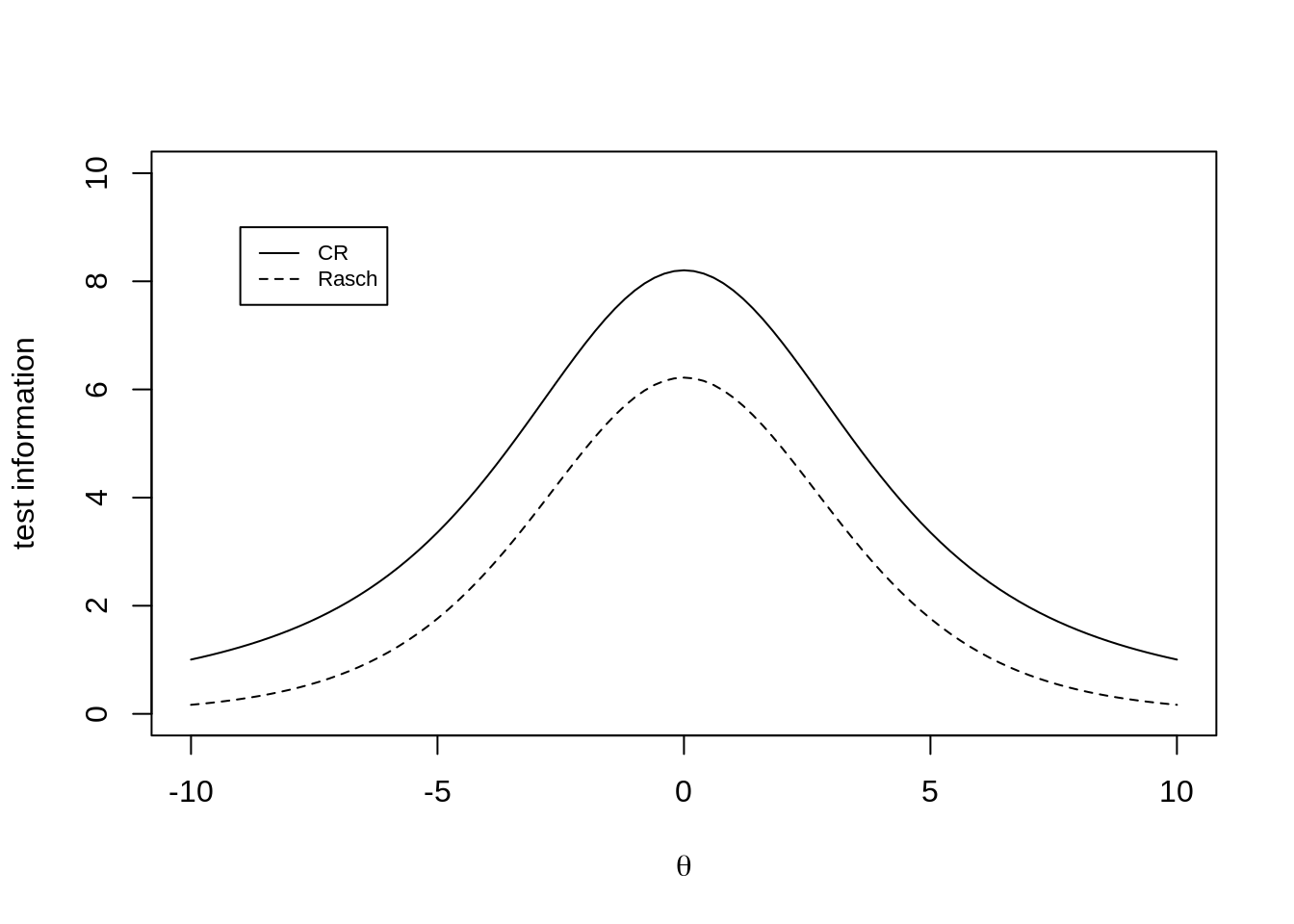
It follows that the information provided by the first binary response, \(1/16\), is already \(75\) percent of what can be achieved under the CRM. We illustrate this with the next plot. Adding a second one would raise this to \(93.75\) percent, a third to \(98.44\) percent, etc. This suggests that three dichotomous items will suffice to capture most of the information in the continuous responses.

The current version of dexter does not allow different items to share the same difficulty parameter, such that data with more than one constructed item cannot be analyzed presently. However, we have some news. dexter may soon have a little brother (or sister) dedicated to the analysis of response times, and models like the CRM will find their natural place there. We have the feeling that the use of response times in practical testing is lagging behind the current state of the methodology, and does not sufficiently exploit the wealth of information they contain. A companion to dexter with the same slant towards the practitioner is probably overdue.
And there is more, much more. The insights in the Maris (2020) and Deonovic et al. (2020) papers lead far beyond traditional testing and into the world of integrated learning systems with their specific concerns of cold starts, ability trackers, and so on. But it would take many more blogs and papers to give proper idea of the full potential – so, for now, we say: Happy New Year!
References
Boeck, P. De, and Minjeong Jeon. 2019. “An Overview of Models for Response Times and Processes in Cognitive Tests.” Frontiers in Psychology 10. https://doi.org/10.3389/fpsyg.2019.00102.
Deonovic, Benjamin Enver, Maria Bolsinova, Timo Bechger, and Gunter Maris. 2020. “A Rasch Model and Rating System for Continuous Responses Collected in Large-Scale Learning Systems.” Frontiers in Psychology 11: 3520.
Dirkzwager, Arie. 2003. “Multiple Evaluation: A New Testing Paradigm That Exorcizes Guessing.” International Journal of Testing 3 (4): 333–52.
Finetti, Bruno de. 1965. “Methods for Discriminating Levels of Partial Knowledge Concerning a Test Item.” British Journal of Mathematical and Statistical Psychology 18 (1): 87–123.
Maris, Gunter. 2020. “The Duolingo English Test: Psychometric considerations.” DRR-20-02. Duolingo. https://duolingo-papers.s3.amazonaws.com/reports/DRR-20-02.pdf.
Maris, Gunter, and Han van der Maas. 2012. “Speed-Accuracy Response Models: Scoring Rules Based on Response Time and Accuracy.” Psychometrika 77 (4): 615–33.
Partchev, Ivailo, and Paul De Boeck. 2012. “Can Fast and Slow Intelligence Be Differentiated?” Intelligence 40 (1): 23–32. https://doi.org/https://doi.org/10.1016/j.intell.2011.11.002.
Settles, Burr, Geoffrey T. LaFlair, and Masato Hagiwara. 2020. “Machine Learning–Driven Language Assessment.” Transactions of the Association for Computational Linguistics 8: 247–63.
Verhelst, Norman D. 2019. “Exponential Family Models for Continuous Responses.” In Theoretical and Practical Advances in Computer-Based Educational Measurement, edited by Bernard Veldkamp and Cor Sluijter, 135–60. New York City, New York: Springer.