Our most distinguished colleague, Norman D. Verhelst, had his birthday a couple of days ago. As a tiny tribute, I offer a lecture I gave a couple of months ago to a bunch of students. They had moderate exposure to statistics, and I have edited it somewhat hastily, so the level is not particularly uniform — sorry, folks.

The RaschSampler (Verhelst, Hatzinger, and Mair 2007) is an R package that allows the user to test a vast array of statistical hypotheses about the Rasch model. It is also a good example of how the statistical testing of hypotheses works, especially in its nonparametric variety.

The theory behind the RaschSampler seems to go back to Georg Rasch himself. In a nutshell: Since the row sums and the column sums in a 0/1 matrix are sufficient statistics for the person parameters and the item parameters in the Rasch model, correspondingly, then any other matrix having the same marginal sums will be just as compatible with the Rasch model in terms of measurement. If we compute a statistic of interest on all matrices having the same marginal sums as our observed matrix, then we can place the statistic for the observed matrix in the distribution of all statistics. The statistic itself can be anything: if you compute the matrix of tetrachoric correlations between all items, divide its seventh eigenvalue by the first, take the log and multiply it by Boltzmann’s constant, it would still work (now, try and derive the asymptotic distribution of this statistic).

Of course, we would like to use sensible statistics — Ponocny (2001) gives many useful examples. And we wouldn’t like to work with all matrices having the same marginal sums, because there are so many of them. But, if we can have a program that produces, efficiently, a representative sample of them, the practical interest is obvious. The key to the problem was given by Verhelst (2008).

As implemented in the RaschSampler package, the procedure produces a prespecified number of unbiased samples from the sample space of all possible 0/1 matrices of the same size and having the same sum and row sums as the user-specified matrix. The user must provide a function that computes some statistic of interest on each of these matrices. It is then trivial to place the statistic for the observed data matrix in the resulting distribution of statistics, and compute the p-value,

For didactic purposes, I start with a function that draws a sample from the bivariate normal distribution. This can be accomplished in a variety of ways but, since the Rasch Sampler is an MCMC method, I have chosen a Gibbs sampler algorithm (see Gelman et al. 2003, 288f):

gibbs = function (n, m1=0, s1=1, m2=0, s2=1, rho=0)
{
  m = matrix(ncol = 2, nrow = n)
  x = y = 0
  for (i in 1:n) {
    x = rnorm(1, m1+(s1/s2) * rho * (y-m2), sqrt((1-rho^2)*s1^2))
    y = rnorm(1, m2+(s2/s1) * rho * (x-m1), sqrt((1-rho^2)*s2^2))
    m[i, ] = c(x, y)
  }
  m
}

m1 and m2 are the two means, s1 and s2 the two standard deviations, and rho is the correlation coefficient. Let us test the function by drawing a small sample of 10 number pairs and computing the correlation:

cor(gibbs(10, rho=.3))

##           [,1]      [,2]
## [1,] 1.0000000 0.4706017
## [2,] 0.4706017 1.0000000

The first time I did this in front of the students, the correlation was close to -.3, so the question is whether there could be a programming mistake. Given a sample size of 10, how compatible is an observed correlation of -.3 with a true value of +.3?

The answer to this question is very similar to the answers provided by the Rasch Sampler. We can create some frame of reference for our observed value by drawing many samples of the same type and size. Each sample will yield another correlation, and these form a distribution. The distribution of the results from all possible samples of the same type and size is called sampling distribution, and its standard deviation is known as standard error. Obviously, we cannot obtain the whole sampling distribution as there are infinitely many samples of size 10, but we can do with a largish sample, as long as it is drawn in an impartial way. In R, we can use the replicate function:

ten = replicate(1000, cor(gibbs(10, rho=.3))[2,1])
hist(ten)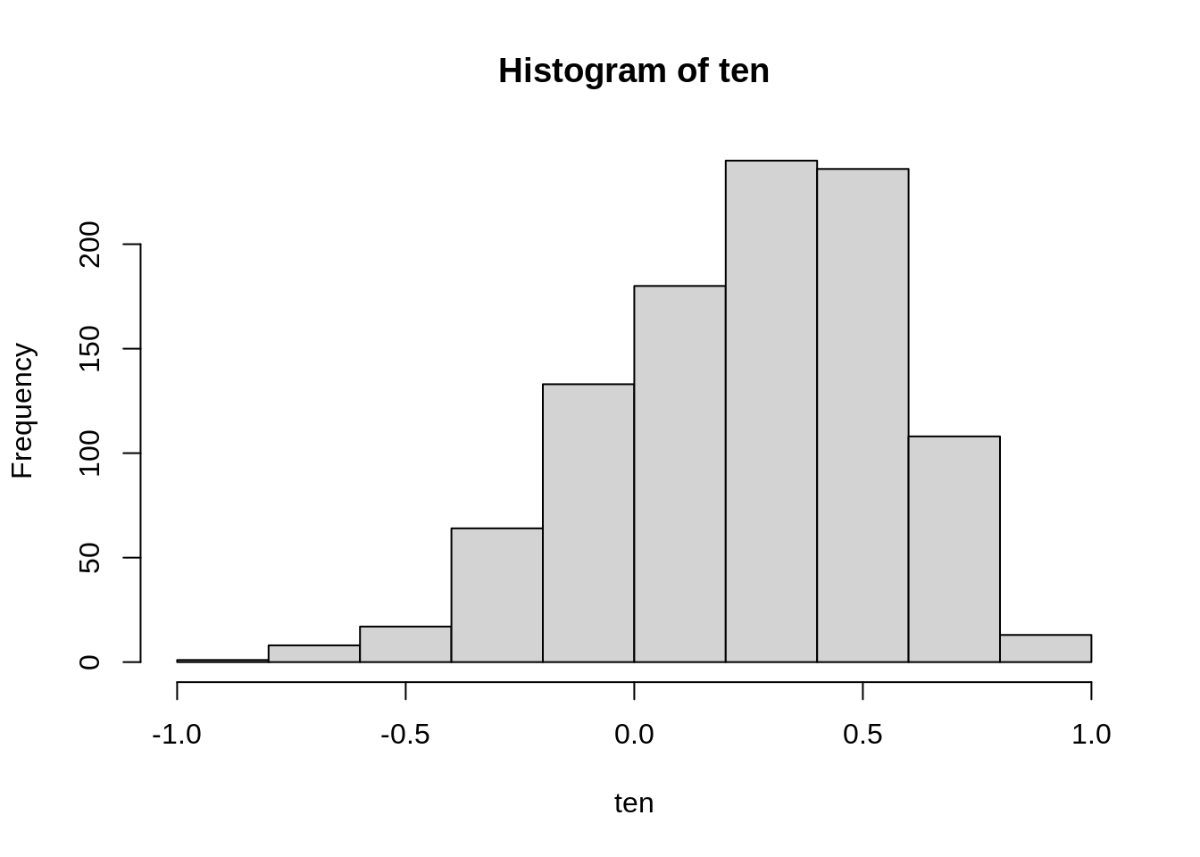

We see that the sampling distribution is skewed, with a longer left tail. The most often observed values seem to be around the true value of 0.3, so samples of size 10 seem to work well on the average. However, the standard error (the standard deviation of the sampling distribution) is so large that an observed value of -.3 should not come as a huge surprise; in fact, we have observed, with various probability, values in the whole admissible range between -1 and +1.

If we repeat the experiment with 1000 samples of size 100, we get:

hundred = replicate(1000, cor(gibbs(100, rho=.3))[2,1])
hist(hundred)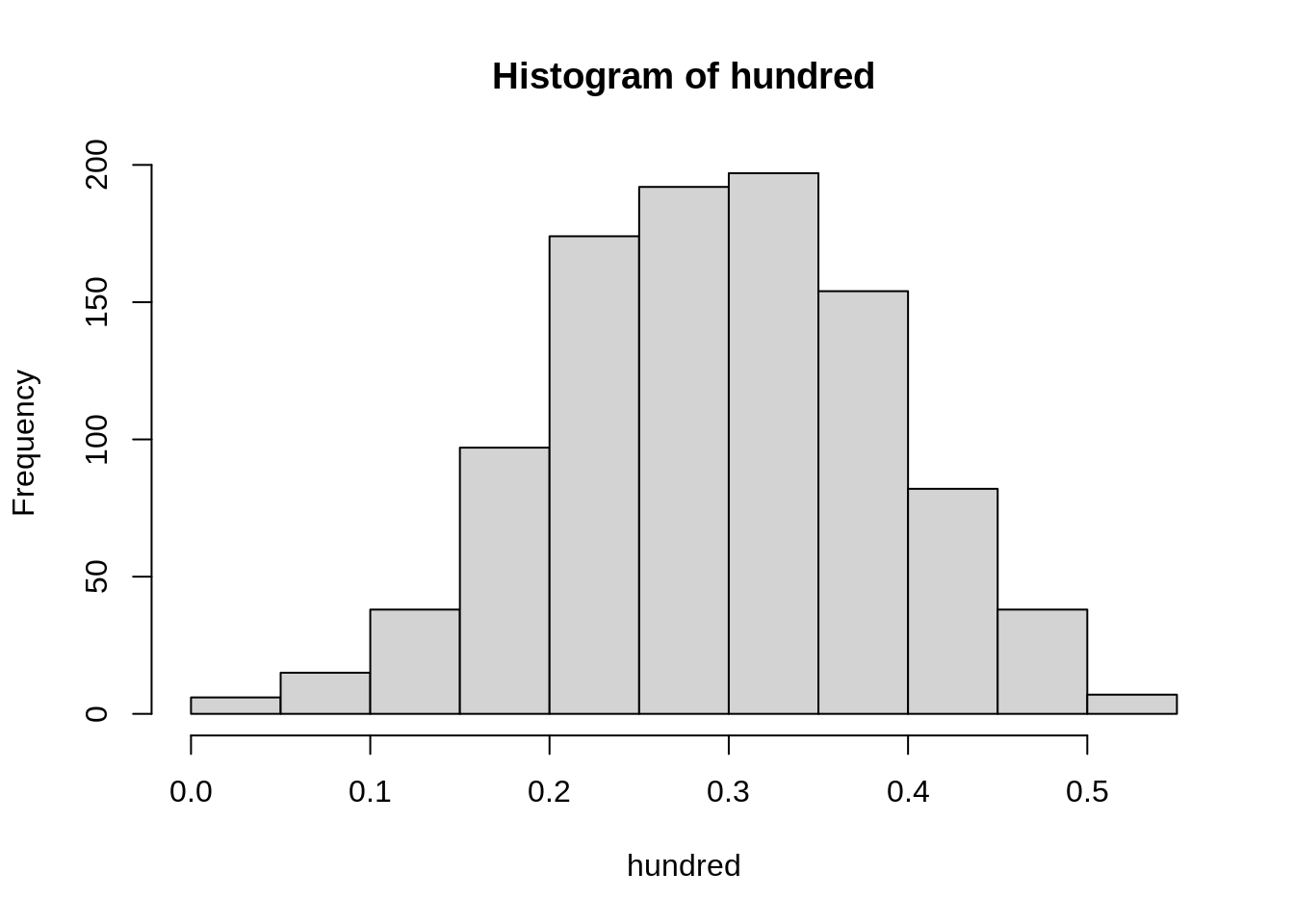

Again, the samples seem good on the average, but now they have more promise for the individual estimates as well, as these do not stray so strongly from the true value. In practice, we will only draw one sample, and we will never know our actual error but, by planning the sample size, we will know what risk we have taken in what is essentially a game of fortune. If we are rich enough to afford a sample of 1000, we will barely observe any correlations outside of the range 0.25 to 0.35.

Let us do an alternative display of the distributions. Instead of histograms, we will plot the empirical cumulative distribution functions (ECDF). These show, on the vertical axis, the probability of observing a value smaller than or equal than the argument on the horizontal axis. Graphs of this type are less popular than histograms but are in fact much more convenient. Observe how much easier it is to compare two (or more) distributions. We could have plotted the two histograms on top of each other but the plot would be very busy.

plot(ecdf(ten), main='ECDF')
plot(ecdf(hundred), col=2, add=T)
abline(v=.3, lty=3)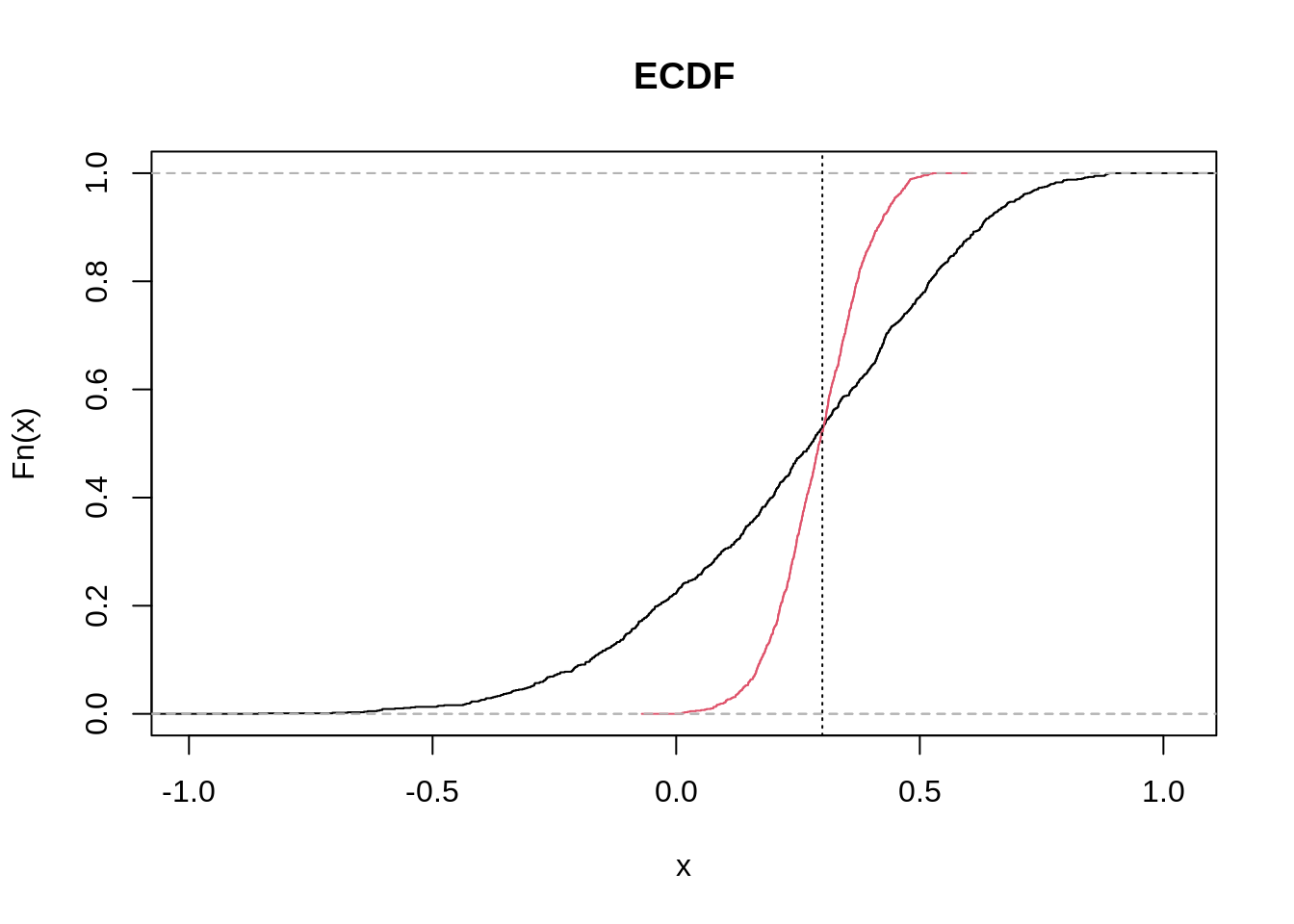

The two curves cross approximately at the true value of 0.3. The smaller the standard deviation, the steeper the curve. Note how an observed value of -.3 is compatible with samples of 10 (black curve) but barely with samples of 100 (red curve).

Placing the observed value of a statistic in the distribution expected under some hypothesis is an instance of statistical testing of hypotheses. In our case, the observed statistic was -.3, and the expected distribution given a true value of 0.3 was obtained by simulation, or sampling. Sometimes we know the theoretical distribution of the statistic under the null hypothesis (typically, the hypothesis that the true value of the statistic is 0, hence the name). Thus, the distribution of a certain function of the correlation coefficient, \(r\), namely \(\frac{1}{2}\ln\left(\frac{1+r}{1-r}\right)\), is normal, and the standard deviation depends only on the sample size, being \(\frac{1}{\sqrt{n-3}}\). However, knowing the distribution of a statistic under the nulll hypothesis is a luxury that we not always can afford. Consider, for example, the hypotheses that:

• the correlation of a particular item with the sum score is significantly lower (or higher) than expected under the Rasch model
• the assumption of unidimensionality of the test is probably violated
• women who have the same overall level of verbal aggression as men tend to give positive responses to certain questions about verbal aggression less frequently.

Let us tackle the second and the third of these. To test whether the assumption of unidimensionality is met, we are going to perform a crude factor analysis. For those unfamiliar, factor analysis and the more straightforward principal component analysis are statistical methods that investigate the inherent dimensionality of a data set. We are going to compute the eigenvalues of the correlation matrix of the items. If the test is unidimensional, there will be one large eigenvalue while all the others must be much smaller, so a viable test statistic is the ratio of the largest eigenvalue to the second largest.

If we want to do factor analysis of a binary matrix, the appropriate correlation coefficiant is the tetrachoric one. It can be quite time consuming to compute, especially if we need to do it many times, so I have programmed the fast approximation proposed by Bonett & Price (reference in the Wikipedia article):

tetra = function (d) {
  n = nrow(d)
  x = crossprod(d,d)
  y = diag(x)
  m = -sweep(x, 1, y, "-")
  o = (x + .5) * (n - x - m - t(m) + .5) / (m + .5) / t(m + .5)
  y = y / n
  w = pmin(y, 1 - y)
  p = (1 - abs(outer(y, y , "-")) / 5 - (0.5 - outer(w, w, pmin))^2) / 2 
  cos(pi / (1 + o^p))
}

We are going to use simulated data, so we need several more functions. The following one-liner simulates data from the Rasch model, given the item parameters, beta, and the person parameters, theta:

simRasch = function (theta, beta) {0+(outer(theta,beta,"-") > rlogis(length(theta)*length(beta)))}

For item parameters, we can use 20 numbers evenly spaced between -1.5 and 1.5:

beta = seq(-1.5, 1.5, length=20)

For person parameters, we already have our gibbs function. We are going to generate bivariate abilities with varying degree of correlation, and have the odd-numbered items measure the first ability and the even-numbered item the second ability. First, let us try a high correlation of .95, such that the test is almost unidimensional:

z = gibbs(999, r=.95)
u = cbind(
  simRasch(z[,1], beta[c(T,F)]),
  simRasch(z[,2], beta[c(F,T)])
)

As mentioned in the beginning, the user of RaschSampler must supply a function that returns the statistic of interest when applied to the original data matrix or to any of the simulated matrices. The following one computes the matrix of tetrachoric correlations, performs the eigendecomposition and returns just the vector of eigenvalues, sorted in descending order:

eigTetra = function(m) {eigen(tetra(m))$values}

Load the library, define some options, and save them in an object, ctr:

library(RaschSampler)
ctr = rsctrl(burn_in = 10, 
             n_eff = 500, 
             step = 10, 
             seed = 123, 
             tfixed = FALSE
)

We are going to sample 500 matrices (n_eff). To avoid autocorrelation, we will use each tenth sample, as specified with the step parameter, which means that the number of generated samples is actually 5000. We have a burn-in period of 10 samples (actually, 100, because step applies here as well). seed is the seed for the random number generator; read the help screen if you must know what tfixed does.

Now, call the rsampler function with the observed data matrix, u, and the control parameters as inputs. The output is a list of 501 matrices: the observed one in position 1, and the 500 generated matrices following.

rso = rsampler(u, ctr)

Next, use the rstats function; the first argument is the list of matrices we generated, and the second is our user-defined function, eigTetra. The result is a list of vectors of eigenvalues. I then use sapply to compute the ratio of the largest eigenvalue to the second-largest:

tet = rstats(rso, eigTetra)
out = sapply(tet, function(x) x[1]/x[2])

Now we only need to place the statistic for the observed table in this distribution. I have written a small function to do this graphically:

rplot = function(x, label="") {
  epv = mean(x>x[1])
  label = paste(label,format(epv,3))
  plot(ecdf(x), main=label)
  abline(v=x[1], lty=3)
  abline(h=1-epv, lty=3)
}

rplot(out)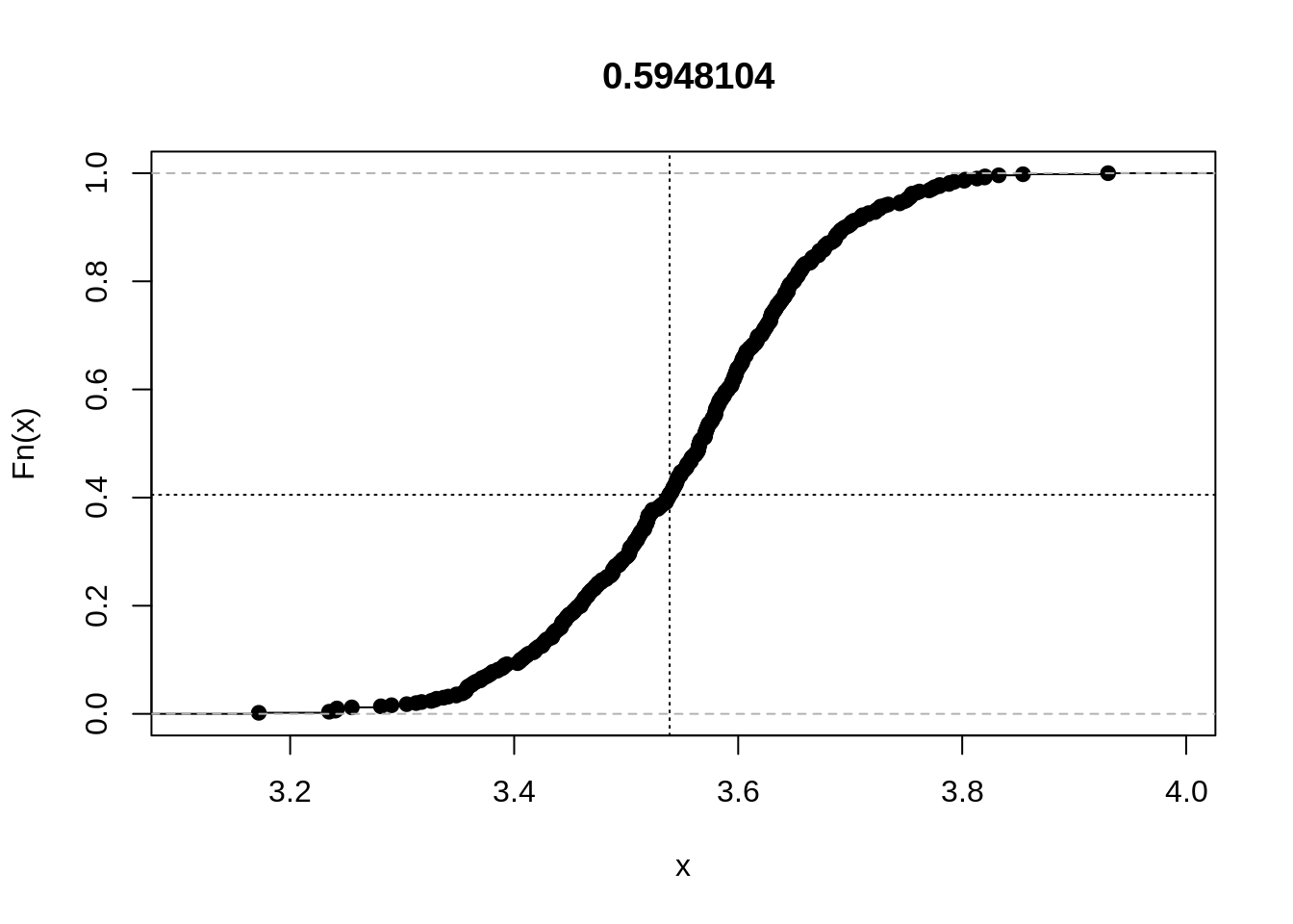

The plot shows the empirical cumulative distribution function of the statistic. The vertical line is drawn at the value of the statistic for the observed data set, and the horizontal line helps place it in the distribution. We see that the statistic is not particularly extreme.

Now, repeat the same, except that we use a low correlation of .35 between the two abilities:

z = gibbs(999, r=.35)
u = cbind(
  simRasch(z[,1], beta[c(T,F)]),
  simRasch(z[,2], beta[c(F,T)])
)
rso = rsampler(u, ctr)
tet = rstats(rso, eigTetra)
out = sapply(tet, function(x) x[1]/x[2])
rplot(out)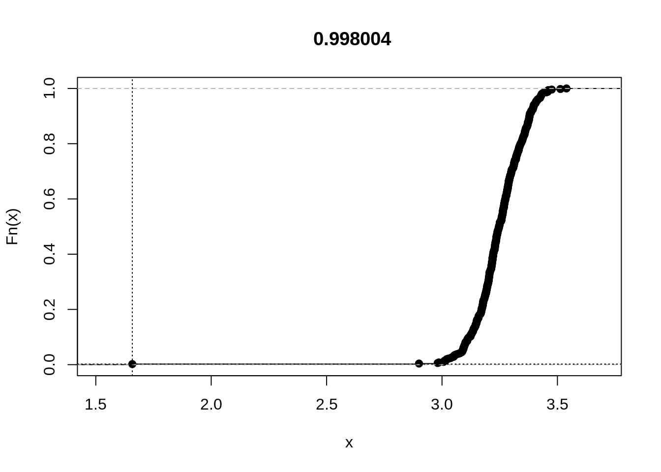

For the second example, let us consider differential item functioning (DIF). In dexter, we have included a popular data set on verbal aggression. 316 subjects (243 women and 73 men) responded to a 24-item questionnaire with questions about four frustrating life situations, two of which are caused by others (‘A bus fails to stop for me’, ‘I miss a train because a clerk gave me faulty information’), while in the other two the self is to blame (‘The grocery store closes just as I am about to enter’, ‘The operator disconnects me when I had used up my last 10 cents for a call’). There are also three types of verbally aggressive behavior: curse, scold, and shout, and two modes: want to do or actually do. Each item can be answered with ‘yes’, ‘perhaps’, or ‘no’. Hence, the design is: In situation [1|2|3|4], I would [certainly|probably|not] [want to|actually] [curse|scold|shout]. We will analyze a dichotomized version with responses ‘yes’ and ‘perhaps’ combined. We know that, whatever their total score on verbal aggressiveness, women tend to score higher than men on a subscore comprising the ‘want to’ items, and lower on a subscore comprising the ‘actually do’ items. In other words, women tend to ‘do’ less than they ‘want to’.

library(dexter)
gender = verbAggrData$gender
d = as.matrix(verbAggrData[,-(1:2)])
doItems = grep('Do', names(verbAggrData)[-(1:2)])
d[d>1] = 1             # dichotomize
rso = rsampler(d, ctr) # sample matrices

For a statistical test based on the Rasch Sampler, we use a very simple statistic as suggested by Ponocny (2001) as Example 4: we simply count the positive responses given by women to any of the ‘Do’ items.

T4 = function(x, grp, fgr, itm){sum(x[grp==fgr, itm])}
out = rstats(rso, T4, grp=gender, fgr='Female', itm=doItems)
rplot(unlist(out))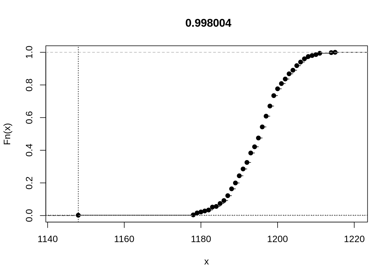

Finally, we take a cursory look at the relationship between sample size and the results from the Rasch sampler. With parametric tests, test statistics increase with sample size, and p-values decrease, so null hypotheses are more likely to be rejected, other things equal. The Rasch sampler is a typical exact, nonparametric test. Let us see what will happen when we apply the last statistic to 50, 100, 200, and all 316 cases:

layout(matrix(1:4,2,2,byrow=T))

rso = rsampler(d[1:50,], ctr)
out = rstats(rso, T4, grp=gender[1:50], fgr='Female', itm=doItems)
rplot(unlist(out), label = "50 cases")

rso = rsampler(d[1:100,], ctr)
out = rstats(rso, T4, grp=gender[1:100], fgr='Female', itm=doItems)
rplot(unlist(out), label='100 cases')

rso = rsampler(d[1:200,], ctr)
out = rstats(rso, T4, grp=gender[1:200], fgr='Female', itm=doItems)
rplot(unlist(out), label='200 cases')

rso = rsampler(d, ctr)
out = rstats(rso, T4, grp=gender, fgr='Female', itm=doItems)
rplot(unlist(out), label='All 316 cases')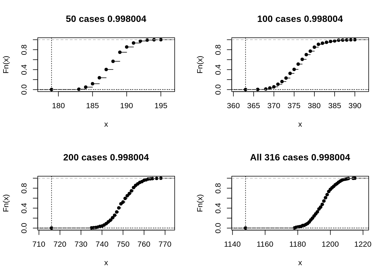

layout(1)

As the sample size increases, the overall value of this particular statistic increases, the relative dispersion decreases, and the statistic for the observed data, always very extreme, gets even farther away. However, the p-value remains the same. The reader might want to experiment with some less extreme examples.

References

Gelman, Andrew, John B. Carlin, Hal S. Stern, and Donald B. Rubin. 2003. Bayesian Data Analysis. CRC Press.
Ponocny, Ivo. 2001. “Nonparametric Goodness-of-Fit Tests for the Rasch Model.” Psychometrika 66: 437–59.
Verhelst, Norman D. 2008. “An Efficient MCMC Algorithm to Sample Binary Matrices with Fixed Marginals.” Psychometrika 73: 705–28.
Verhelst, Norman D., Reinhold Hatzinger, and Patrick Mair. 2007. “The Rasch Sampler.” Journal of Statistical Software 20.